A. Bows, rods and Amontons’ law
We have seen some examples of measurements and simulations of bowed-string transients, and the initial comparison of the two was decidedly disappointing. Something is obviously wrong with the simulation model described so far, and in this section we explore a likely culprit: the approach we have used to characterise the friction force.
Up until now, we have been using a particular model to describe the frictional behaviour between the bow and the string. This model is based on two assumptions: that the friction force is proportional to the normal force (i.e. the bow force), and that during sliding the friction force is a nonlinear function of the sliding speed. The time has come to look carefully at both these assumptions. What is the empirical evidence and/or theoretical understanding on which they are based?
This turns out to be an interesting but tricky question, and it will lead us right up to a research frontier. Most things we have discussed in all the chapters up to this point have been governed by physical principles like Newton’s laws, which are well established and uncontroversial. But friction is different: there is no single underlying theory that has similar status. The mechanism of friction can be quite different depending on the nature of the materials in contact, and in many cases we still don’t know the full story. Most of the time engineering calculations involving friction make use of grossly simplified approximations, but these are not good enough if we want to understand bowed-string transients in detail.
The first assumption, that friction force is proportional to bow force, is often called Amontons’ “law”. It is so familiar to anyone who has studied mechanics or physics at any level that many people are surprised to learn that there is any question about it. But the result is a purely empirical finding, and the generally accepted explanation involves something unexpectedly subtle.
Amontons published his “laws of friction” in 1699 (although in fact this was a re-discovery: they were stated in the notebooks of Leonardo da Vinci some 200 years earlier, but Leonardo never published them). The first two of these laws state that the force of friction is proportional to the applied load, and independent of the apparent area of contact between the sliding surfaces. The original experimental evidence gathered by Amontons and others involved a classic experiment with an object like a brick resting on an inclined plane (such as a wooden plank): the angle of the plank is slowly increased, until the brick starts to slide.
If you were to examine the surfaces of the brick and the wooden plank under a microscope, neither of them would be smooth. Instead, they would be covered with small lumps and bumps known in the jargon as asperities. The result would be something like what is sketched in Fig. 1: actual contact between the two surfaces only occurs near the tips of these asperities. The real area of contact will be much smaller than the apparent area of contact.
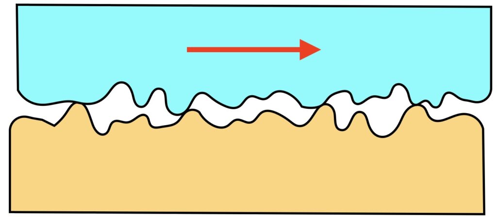
The accepted explanation for Amontons’ laws then goes like this. The friction force is determined by the shear strength of the interface between the two materials, acting over the real area of contact. So under the simplest assumption, friction force is directly proportional to real area of contact. When the applied load is increased so that the surfaces are pressed together more firmly there is some deformation near the asperity tips, with the result that each individual contact gets a bit bigger, and also additional asperities may come into contact. In a classic study by Greenwood and Williamson [1], it was shown that under reasonable assumptions about the statistical description of the surface roughness, the real area of contact ends up being proportional to the applied load. Putting these two things together, the friction force is proportional to the load, as Leonardo and Amontons found.
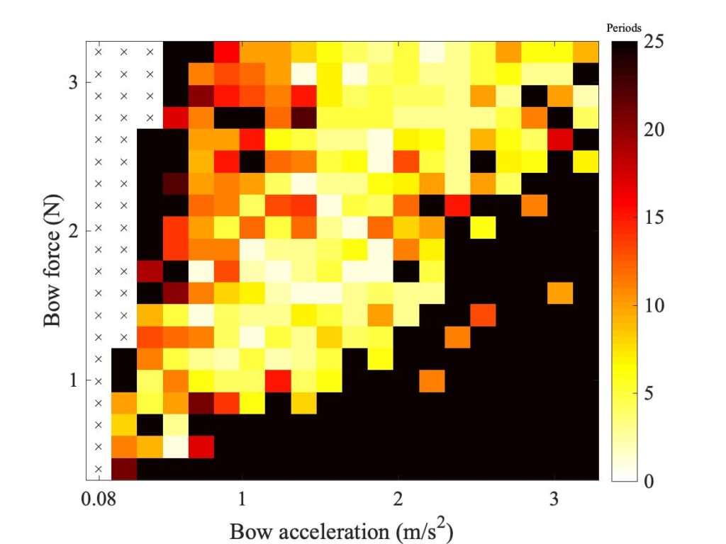
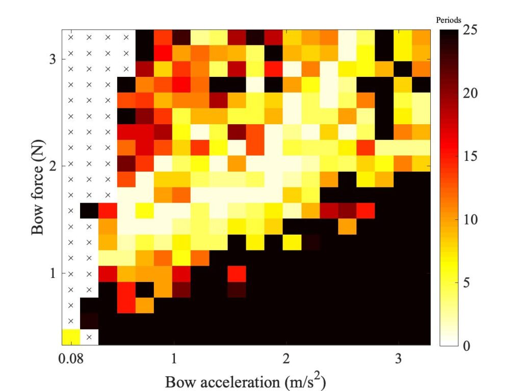
Figure 2 shows a measured Guettler diagram using a real bow in the Galluzzo experimental rig, and Fig. 3 shows the corresponding one measured on the same rig with the rigid rod. The green and magenta lines will be explained in a moment. At first glance, these two plots look fairly similar. They both show a vaguely wedge-shaped region of transients that led to successful Helmholtz motion, and they both include quite a few white or yellow pixels indicating very short transient length. Both show some “speckly” texture, suggesting a degree of “sensitive dependence”.
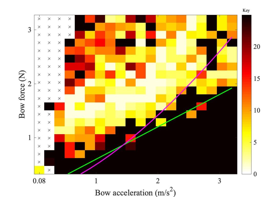
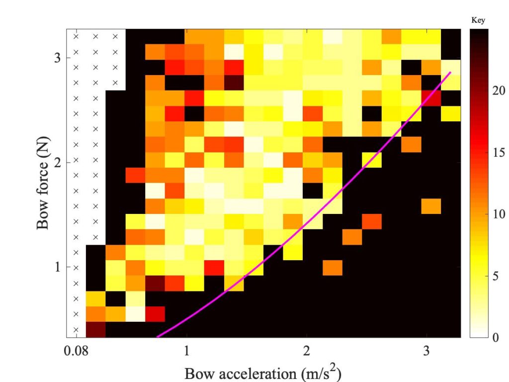
One clear difference between the two figures is in the position and shape of the lower boundary of the region of coloured pixels. Figure 2 shows more black pixels than Fig. 3 in the lower left corner, but the pattern is opposite on the right-hand side: Fig. 3 shows a boundary curve that rises more steeply than the one in Fig. 2.
What does this have to do with the question of whether Amontons’ law holds? Well, in the experiment with the rosin-coated rod we would probably not expect this argument based on rough surfaces to work. When a string is bowed by a rod, the geometry is like two cylinders, crossing at right angles. The apparent area of contact is very small, so the contact pressure (force per unit area) will be very large. Rosin is not a very hard material, especially when it has been warmed up by friction. With this large contact pressure, any asperities that may have originally been present on the surfaces of the rosin-coated string and rod will be squashed flat. The real area of contact will then be more or less the same as the apparent area of contact.
Under those circumstances, the argument based on rough surfaces goes out of the window. Instead, we would expect the material near the contact to behave in a way first described in 1882 by Heinrich Hertz (the same scientist that our unit of frequency is named after). You can find a description of this “Hertzian contact”, and of the Greenwood-Williamson model of rough surfaces, on this Wikipedia page. For a Hertzian contact, the friction force is not proportional to the applied load: instead, it is proportional to the 2/3 power of that load.
So now look again at the Guettler diagram in Fig. 3. Guettler’s original argument suggested that the wedge of short transients would be bounded by a straight line — but he was assuming Amontons’ law. What his criterion really calls for is that the friction force is proportional to the acceleration. If the rod-string contact is Hertzian, the boundary should show bow force proportional to the acceleration raised to the power 3/2: a rising curved line, not a straight line. The magenta line in Fig. 3 shows what that looks like: it doesn’t do a bad job of tracking the lower boundary of the coloured pixels.
Now what about the Guettler diagram measured with a real bow? We can make a guess. The ribbon of bow-hairs must produce an effect which is rather like the rough surfaces of Greenwood and Williamson. Each individual contact between the string and a single hair might play the role of an asperity contact. As the bow force is increased, more hairs might come into contact with the string. The result would be to resurrect something like Amontons’ law. If that were exactly true, the boundary would be a radial straight line in the Guettler diagram. The green line in Fig. 2 shows an example. It doesn’t track the boundary very well at low values of bow force, where perhaps things are more complicated, but with the eye of faith it does a reasonable job of tracking the boundary at higher forces. Figure 2 also repeats the magenta line from Fig. 3: it is obvious that this line rises far too steeply to be consistent with the pattern of these measurements. A similar contrast can be seen when comparing the plots for other values of $\beta$ shown in Figs. 7 and 9 of section 9.5: the real bow shows a straight-sided wedge, while the rod shows a “curving wedge”.
This effect might, just possibly, be the main reason for using the complicated arrangement of a ribbon of horsehairs to make a bow. A bow could instead be strung with something like a large-diameter gut string (rather in the style of an archery bow). The string could be chosen to have the same total mass as the horsehair bundle, so that if it was adjusted to the same tension it would have the same bouncing frequency. Such a string will accept a coating of rosin just as well as horsehair does. But, despite matching several aspects of the mechanical behaviour, it is virtually impossible to play an instrument with such bow. I have tried the experiment, and there is an overwhelming impression that you can’t press hard enough to get the string response you are expecting. That impression would be a natural consequence of the contrast between Hertzian contact and Amontons’ law. (At least, this is what happens when a modern bow stick is used to hold the gut string — things might be a bit different with an up-curved bow stick as used in earlier times.)
B. The friction curve model
Now to return to the second assumption, that friction force is governed by some function of the sliding speed: the “friction curve model”. Our starting point is the measurement we saw earlier, repeated here as Fig. 4.

Looking at this plot, it seems obvious that the friction force varies, rather dramatically, with the sliding speed. But we have to be careful to avoid a trap here. This plot shows the results of a particular type of measurement: for each separate data point, steady sliding was imposed at a particular speed, and the friction force was measured. Sliding speed is the only variable, so of course we can plot the measured forces against the speeds and we are bound to get something looking like a friction curve.
But now suppose we do a different measurement, in which the sliding speed varies in time (as it does with the actual bowed string). Do the results from Fig. 4 prove that the friction force is determined, moment by moment, by the instantaneous value of the sliding speed? Absolutely not! Other factors might come in, to do with the history of the motion. Figure 4 only says that if the speed stays constant for long enough, the force should settle down to the value plotted there. To resolve this question, we need to do measurements of a different kind.
It is not easy to observe the friction force directly during stick-slip vibration of a bowed string, or indeed of any other stick-slip system like a squealing vehicle brake. It is very difficult to insert any kind of force-measuring sensor right in the contact region, without drastically changing the behaviour. Instead, ingenuity must be exercised to design an experiment in which the friction force can be reliably inferred from measurements of some kind elsewhere on the vibrating structure.
C. The Smith and Schumacher experiments
For the case we are interested in, when the friction is mediated by violinist’s rosin, two different experiments of this kind have been carried out. The first, by Jonathan Smith [2], made use of a cantilever-like mass-spring oscillator. Once the effective mass, stiffness and damping of the device have been found by calibration tests, the motion of the mass during a stick-slip vibration can be measured and the friction force can be reconstructed by substituting the displacement, velocity and acceleration into the equation of motion of the oscillator.
The second experiment used an actual bowed string. Bob Schumacher designed a rig in which a violin E string was bowed by a glass rod which had been coated in rosin [3,4]. The rosin was dissolved in a solvent, then a rod was slowly drawn up out this solution, leaving a thin film of rosin after the solvent had evaporated. At both ends of the string, force-measuring sensors of the kind described in section 9.1.1 were inserted. With a bit of ingenious processing in the computer, these two force signals can be combined to give estimates of the string velocity and the friction force at the bowed point. The next link gives a few details about how this can be done.
The Schumacher experiment gives the most illuminating information for our purpose, so we will show some results from this rig. Figure 5 shows a few cycles of the inferred waveforms of velocity (upper plot) and friction force (lower plot). The string was executing Helmholtz motion in this example. The pulses of slipping, with negative velocities, are clear. In between, the episodes of sticking do not show a velocity that is exactly constant. Small ripples in this waveform arise because the string can roll on the “bow”, as described in sections 9.5 and 9.5.3.

Now if we take these waveforms of velocity and force and we plot one against the other, we get the result seen in Fig. 6. There is a more-or-less vertical stripe at the right-hand side, showing the intervals of sticking. But during slipping, instead of a single friction curve we see a loop. The path around this loop moves anti-clockwise. The friction force is highest at the start of slipping (or in fact just after the start of slipping), then it falls as the slipping speed increases. But on the way back towards the sticking line, the force remains much lower than the maximum value on the way out. The details of the loop shape can vary in different bow strokes, but the qualitative behaviour is always very similar to this plot. Furthermore, Jonathan Smith’s experiment also gave very similar results, despite using a very different vibrating system.

The conclusion is that the friction force is not simply determined by the sliding speed: you get a different answer depending on whether the speed is increasing or decreasing. Rosin does not follow the kind of friction-curve model we have been assuming up to now. So what is going on? We should step back a little, and ask what is special about rosin. Why do violinists use it in the first place? Indeed, it is not only violinists: there are many bowed-string instruments around the world, and there are also other musical instruments which make use of stick-slip vibration, for example friction drums. Players of all these instruments coat their bowhair, or their hurdy-gurdy wheel, or in the case of friction drums their fingers, with rosin.
D. Temperature sensitivity of rosin behaviour
Rosin is a natural material, obtained from various species of pine tree. The raw tree resin is separated using distillation or solvents into a liquid component called “spirit of turpentine” and a solid component, which is rosin. It is manufactured in industrial quantities, because it has many uses: it is used in making soaps, printing inks, paper, adhesives, and many other applications. It is also frequently used for its high friction: not only for violin bows, but also to give dancers, weightlifters or baseball players a firmer grip on things.
Violin rosin is a clear, brittle material at room temperature: if you drop a block on the floor it is likely to shatter. But if you hold it in your fingers for a minute or two, it soon becomes sticky. It is a type of material known technically as a glass. As any glass-blower knows, if you heat ordinary glass up it does not show a sharp melting point at which it suddenly becomes a liquid (like melting ice). Instead, there is a broad range of temperatures over which the glass softens progressively. By holding the temperature in this range, the glass-blower can shape and mould it into laboratory glassware or decorative drinking glasses.
Rosin behaves in a similar way, but the changes happen at a lower temperature than with glass. The softening range of temperatures, usually characterised by the glass transition temperature marking the middle of the range, is not very far above room temperature. What this means is that the mechanical properties of rosin change rather quickly with a relatively small rise in temperature. As the temperature rises, the rosin becomes softer, so that the force required to deform a layer of rosin goes down. This could be the origin of the behaviour seen in Fig. 4. When a rosin-coated bow or rod is forced to slide across another object (such as a violin string), heat is generated. The faster the sliding, the hotter the rosin becomes, and the lower is the resulting friction force. So the friction force would indeed vary with the sliding speed, but only indirectly. The real cause of the variation would be a change of temperature.
The idea that the friction force is strongly influenced by temperature, rather than sliding speed as such, gives an immediate qualitative explanation for the loop seen in Fig. 6. Heat is generated during episodes of sliding, but very little is generated during episodes of sticking. So think what will happen during a cycle of Helmholtz motion. At the end of a slip, the rosin will be relatively warm and so the friction will be low. But during the relatively long sticking interval, the heat has a bit of time to diffuse away into the body of the string and bow. So by the time the Helmholtz corner arrives back to trigger the next slip, the rosin layer has cooled down a bit, and the friction force is higher. As it slips, the rosin heats up rapidly and the friction falls. The result is a loop in the velocity—force plane, just as we saw in the measured results.
What this description amounts to is a suggestion that the rosin melts a little and re-freezes during every cycle of the string’s vibration, several hundred times a second. Is that really credible? Remarkably, we can get some direct evidence for this from the Schumacher experiment. We can use one of his glass rods for just a few bow strokes in the apparatus, rotating it a bit each time so that a different part of the rosined surface is used. We can then take that rod and look at it in the scanning electron microscope, and we see visible tracks left by the string’s vibration.
Figure 7 shows an example. The featureless grey background is the very smooth surface of the rosin coating on the glass rod. Running across this background we can clearly see three tracks, made up of a fairly regular row of little vertical lines. Each of those lines is the “footprint” of a single sticking event in the string’s vibration. The orientation of the string was vertical in this image, and the rod has been moved in the horizontal direction when performing the bow stroke. The three tracks have been created by three separate bow strokes.

Figure 8 shows a zoomed view of a portion of one of these tracks, and Fig. 9 shows an even closer view. Each of the vertical scars in the track shows churned-up rosin. This is the result of the string rolling back and forth a little during that sticking interval. But then the string slips rapidly across the surface of the rod, and we can see very clear evidence that the rosin has been partially melted: look at the streaks on the left-hand side of Fig. 9. These are surely “threads” of hot rosin, drawn out by the string as it slipped across the surface.


Figure 10 shows a low-angle view, to give a different perspective on the terrain revealed by these images. The churned-up texture created by the rolling string during the sticking event which caused the scar in the middle of the image is particularly clear here.

There are standard laboratory measurements that can give information about the mechanical properties of rosin as a function of temperature. As a first step, the usual way to determine the glass transition temperature is with a device called a “differential scanning calorimeter”. This measures the amount of heat absorbed by a small sample of rosin (or whatever material is being tested), as the temperature is slowly raised. Whenever a material undergoes a phase transition from solid to liquid, or from liquid to gas, heat energy must be supplied in the critical temperature range. The resulting peak in the heat absorbtion identifies the temperature of the transition. In the case of a glass transition the peak is quite broad, but its highest point can still be used to put a number on the glass transition temperature.
But we are most interested in mechanical properties, rather than thermal properties as such. For this, we can use a device called a “rheometer” which measures the force needed to deform a layer of the material. The specific deformation we are interested in is shear, because a sliding frictional contact requires shearing between the two surfaces. Figure 11 shows some results of measurement of the shear viscosity of two different types of commercial rosin for bowed instruments, which represent the extremes of available behaviour. The temperature has been varied slowly during the test. The red points are for violin rosin, of the kind we have been talking about so far. The blue points are for a brand of rosin aimed at double bass players. This bass rosin is supplied in a pot: unlike violin rosin, which is supplied in a solid block, the bass rosin will flow, slowly, at ordinary room temperatures so it needs to be prevented from getting away.

The glass transition temperatures of the two types of rosin are shown by vertical dashed lines in corresponding colours: $16^\circ$C for the bass rosin, and $49^\circ$C for the violin rosin. The variation of viscosity with temperature reflects this difference: the two curves have very similar shapes, but they are separated along the temperature axis by approximately the difference of these two temperatures. These plots make it rather clear why the bass rosin needs to be kept in a pot: it is already above its glass transition temperature at normal room temperature.
There are two things to notice about this viscosity plot. First, there is a gap in the sequence of red points. This is simply because two different types of rheometer were needed to cover temperature ranges where the material was “solid” and “liquid”. But it is easy to see that the two would join up if the intermediate range of temperature could have been tested. The second thing to note is the vertical scale. A logarithmic scale is needed for the viscosity because the values have changed by almost 7 orders of magnitude over this range of temperature. When I said that the mechanical properties of rosin changed sensitively with small changes in temperature, I was not joking!
E. A thermal model of friction
The next step is to try to extend the computer simulation model to incorporate temperature-dependent friction. First, we need to calculate the temperature in parallel with simulating the string motion. The simplest version of such a calculation is easy to describe. Figure 12 shows a schematic close-up of the contact region of rod, string and rosin. The rod (being used as a bow as in the Galluzzo or Schumacher experiments) carries a layer of rosin. It is moved across the string, seen in cross-section in the sketch. There will be a small “contact footprint” between rod and string, with a size that depends on the diameters of rod and string, and also on the normal force (as discussed at the start of this section). In that footprint region, the rosin will be warmer than ambient temperature, indicated by the red patch.

To work out the temperature in this contact patch, we can do a “heat balance” calculation. There are four effects to consider. Heat is being generated by friction, at a rate which is simply the product of the friction force and the speed of relative sliding between the two surfaces. Heat is being lost by two mechanisms. First, there is diffusion of heat by conduction into the bodies of the rod and the string. The second mechanism is associated with the moving rod: cold rosin is carried into the contact area, while warmer rosin moves out at the other end, taking some heat away with it. Finally, there is a term associated with changes in the heat stored in the red contact region: if the temperature is rising, then heat is being added; if it is falling, heat is being removed. Putting these four things together yields a governing equation that we can solve in the computer, alongside the simulation of the string’s motion. In the unlikely event that you are keen to see the gory details, they are explained in reference [2] (you can find a PDF at number 61 in the list here).
Now for the difficult part: we need to choose a specific model for exactly how the friction force is influenced by the temperature. So far, I have been talking as if the force will only depend on temperature, but this is rather misleading. One thing we definitely know about any friction force is that it always opposes the sliding motion. It must change sign if the sliding direction is reversed — but of course the temperature will be the same, regardless of the direction of sliding. So the friction “law” we are looking for must involve the sliding velocity as well as the temperature, in some way. We don’t really have enough experimental data to determine the correct answer, so we need to resort to a bit of guesswork and empirical exploration.
The simplest model, and the one that has been most extensively investigated, is to assume that the coefficient of friction is a function of temperature alone [6, 7]. This coefficient would be multiplied by the sign of the sliding speed ($+$ or $-$) to give the necessary reversal of friction force when sliding reverses. We can use the measurement from Fig. 4 to infer what the variation with temperature must be. The same computer code can be used to simulate the steady sliding experiment, and thus obtain the contact temperature as a function of sliding speed. This can be used to convert the results of Fig. 4 into a function of temperature: the result is shown in Fig. 13. These results are based on violin rosin similar to the red points in Fig. 11, so it probably has a similar glass transition temperature, around $49^\circ$C. It is reassuring to see that this temperature falls near the middle of the downward slope in Fig. 13.

Armed with this function of temperature, we are ready to incorporate the thermal friction model into our bowed-string simulation. Figure 14 shows an example of a Guettler constant-acceleration transient, simulated in this way. Specifically, it is the case corresponding to the pixel (10,14) in the Guettler plots seen in section 9.5 (10th acceleration from the left, 14th force from the bottom, bow position $\beta=0.0899$). The red curve shows the new simulation, while the black curve in this figure shows the corresponding measured bridge force. In this case, both of them lead to the Helmholtz sawtooth, after a rather short transient.

Figure 15 shows the corresponding computed temperature variation. The mean temperature is predicted to rise to some $70^\circ$C, and in every cycle of the final Helmholtz motion there is a fluctuation by some $30^\circ$C. This certainly seems like a big enough change to account for the appearance of the tracks on the glass rod seen in Figs. 8—10: the rosin looked “melted” during slipping, but semi-solid during sticking.

However, we only learn a rather limited amount by looking at a single transient like this. The next step is to use the new model to scan a family of transients and construct a Guettler diagram. Figure 16 shows an example, chosen to match the cases we saw in Fig. 7 of section 9.5, which is reproduced here as Fig. 17 for easy comparison. It is immediately obvious that the new model behaves quite differently to the friction-curve model. It has produced a fairly solid patch of colour (marking cases that led to Helmholtz motion), in contrast to the “spotty” texture of the friction-curve case.


So far, so good: but the patch of colour in Fig. 16 is nowhere near as big as the corresponding patch in the measured Guettler diagram. We have already commented that a player of the friction-curve “cello” would find their job almost impossible: every pale pixel marking a good, fast transient is not far from some black pixels. This means that if the cellist tried to repeat a successful bow stroke, they are likely to be frustrated by sensitivity to small details of the gesture. The “thermal model cello” of Fig. 16 might be slightly preferred: there is a region of the Guettler plane where virtually every transient gives a successful outcome, with relatively gradual variations in transient length. However, the real cello would surely win hands down in this playability comparison: it offers a far larger range of transients that “work”. From the point of view of a beginner, this means that it is easier to perform a bow gesture that is not a disaster. From the perspective of an expert, the larger available area of the plane will open up a wider “sound palette” of musical possibilities.
F. Improving the thermal model
So can we do any better than this? By drawing inspiration from an aspect of the measurements, we can construct an enhanced version of the thermal friction model. Comparing the two waveforms in Fig. 14, we can see one qualitative difference at the very start of the string’s vibration. Both waveforms begin with a similar rising curve. What is happening here is that the string is sticking to the bow, so it is being pulled to one side by the accelerating motion of the bow. The motion we are interested in can only begin after the first moment of release, when slipping starts. In the measured waveform (in black), that first release happens with a jump. The simulated waveform in red shows no such jump. Furthermore, as explained in the next link, this version of the thermal friction model can never show a jump.
There is a simple way to enhance our friction model to allow the possibility of jumps. The argument is explained in the side link: it involves combining the ideas of the friction-curve model and the thermal model, so that the friction force is determined by a combination of the temperature and the sliding speed. By systematically analysing the initial jumps in a set of Guettler measurements, a particular function of sliding speed can be found, which should give the best chance of matching the pattern of jumps. Interestingly, when this approach is applied to the Galluzzo measurements the results with the rosin-coated rod give a significantly different answer from the results with the normal cello bow.
In the course of developing this enhanced model, something else was discovered. So far, we have been using a particular curve-fit to the steady sliding friction measurements, the curve shown in Fig. 4. This fitted function has been used in many studies of bowed strings, but it is not the only possibility, and making a different choice turns out to affect the simulation predictions. Figure 18 shows the same data as Fig. 4, but over a larger range of sliding speed. The red curve is the approximation used up to now; the green curve is an alternative, proposed and explained in the previous link. Both curves fit the measured points well, but they behave quite differently at higher sliding speeds. Something very much like the green curve is needed in order to allow the enhanced friction model to work properly. But using this curve will also change the predictions of the friction curve model and the original thermal model, as we will now see.
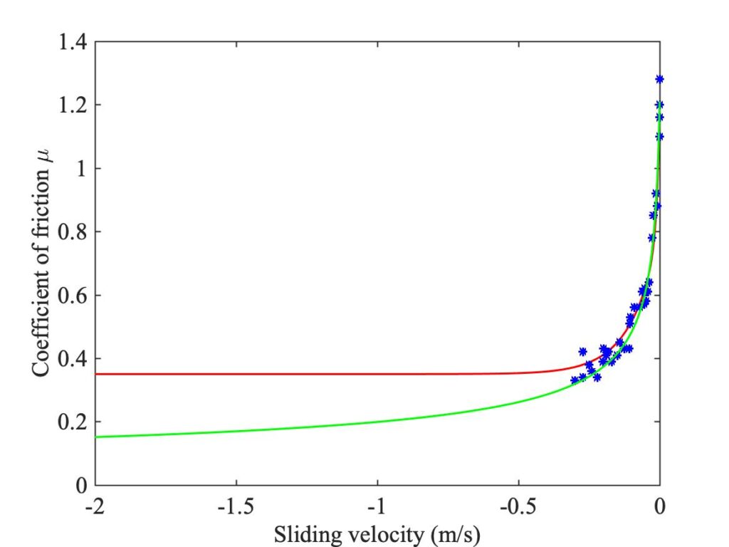
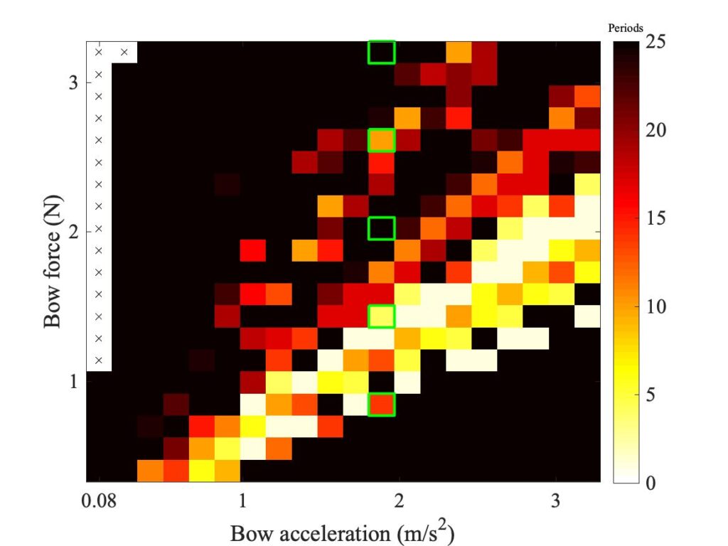
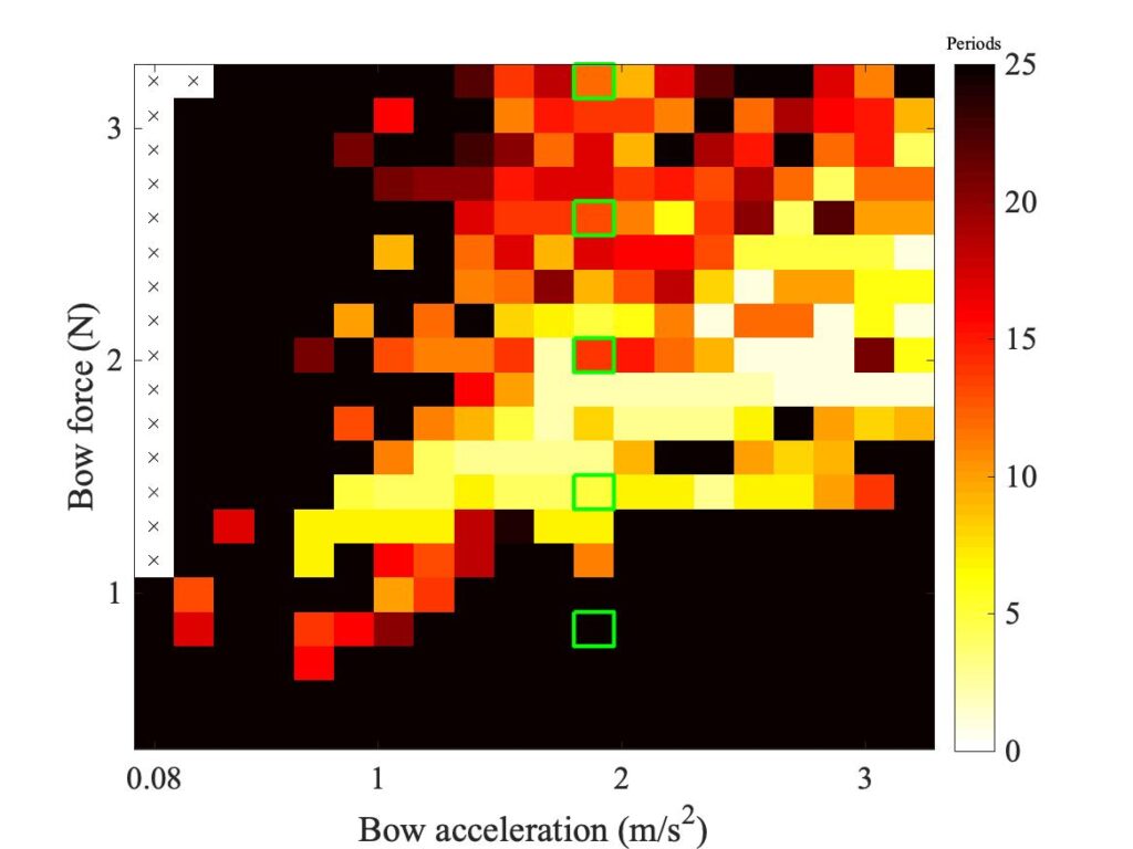
Figure 19 shows a new set of Guettler diagrams. On the top row are the two measurements, with the rod (left) and bow (right). The rod measurement is a repeat of the left-hand plot of Fig. 17. The other four plots are based on simulations by the different friction models, using the new curve fit: the middle row has the friction curve model on the left and the original thermal model on the right, then the bottom row has two cases using the enhanced thermal model: on the left using the fit to the Galluzzo data for the rod, and on the right using his data for the bow. The plot for the friction curve model is somewhat different from the one seen in Fig. 17, but the plot for the original thermal model is very different from Fig. 16: it now shows a much larger region of coloured pixels.
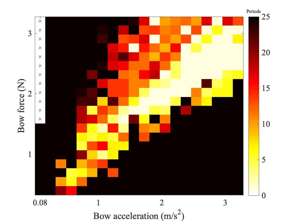
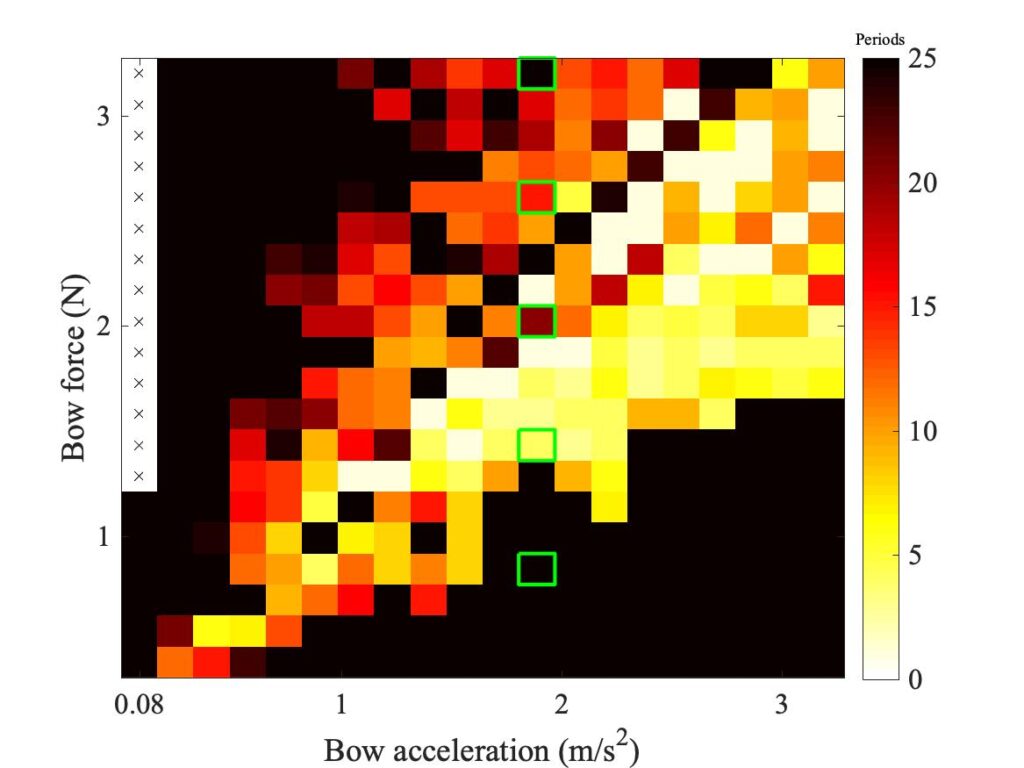
The right-hand plot for the new enhanced model is rather similar to the plot for the original thermal model above it: on this evidence, the new model doesn’t look particularly “enhanced”. But both look much closer to the corresponding measured case on the top right than the plot in Fig. 16: it looks as if the new curve fit to the steady sliding measurements, shown in Fig. 18, has made a big difference, which comes through in both models. In a moment we will explore further into whether the “enhanced” model deserves its name, but before that we can show an interesting illustration of sensitive dependence and speckliness.
Figure 20 shows four more Guettler diagrams, all based on the bottom right plot from Fig. 19, but with very small perturbations to one of the model parameters. They all give similar results, but the individual speckles vary just as we saw in the measured data in Fig. 14 of section 9.5. This is “sensitive dependence” in action. If we take these five variants of the same model, and combine them to look for the shortest transient in each pixel, the result is shown in Fig. 21. The speckled texture has largely vanished, leaving a rather smooth graduation of colour which shows very clearly the pattern suggested in Fig. 6 of section 9.5 on the basis of Schelleng’s bow force limits. There is a core wedge of very short transients. Below it is a patch of yellow, indicating only slightly longer transients until the minimum bow force line is reached. Above the core wedge, though, we see a progressive shift through oranges to reds as expected from the behaviour of the maximum bow force limit.
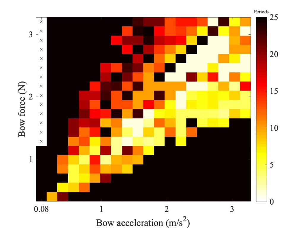
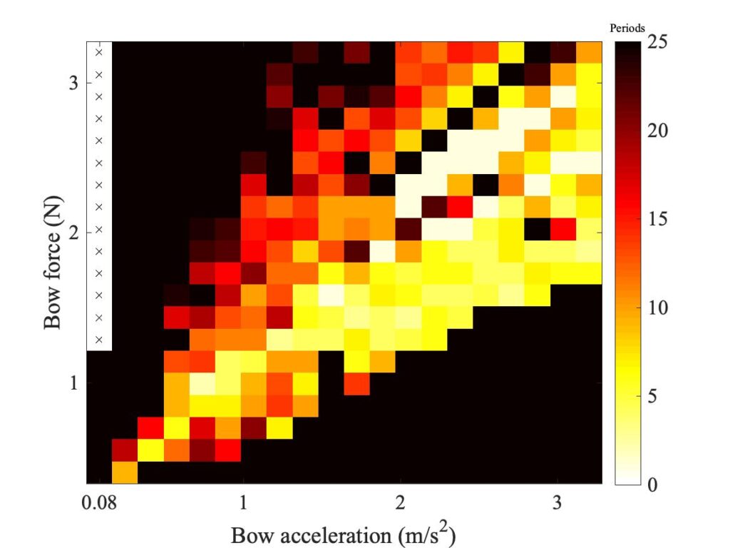
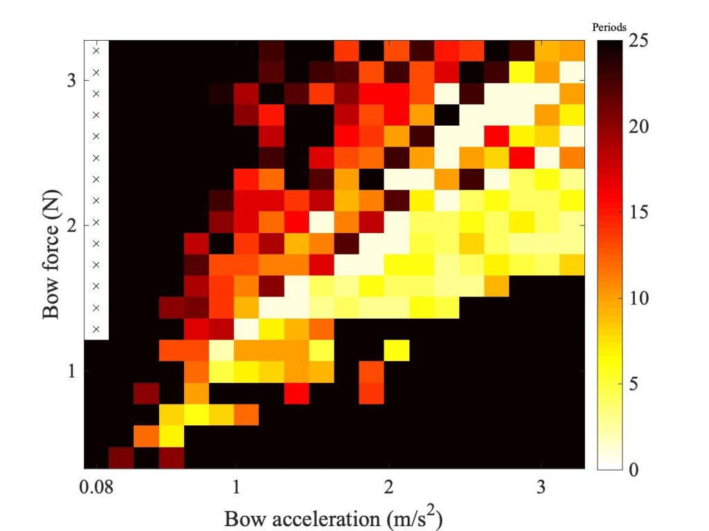
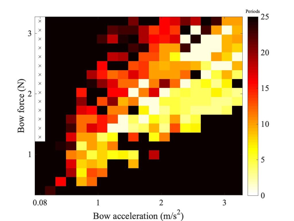
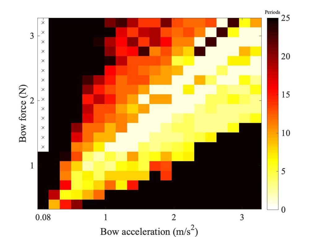
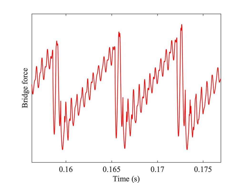
The conspicuous line of black pixels in the top right-hand corner indicates cases of persistent “double flyback motion”, one of the other possible ways a bowed string can vibrate instead of Helmholtz motion. The name comes from the characteristic shape of the bridge force waveform, illustrated in Fig. 22 from one of these simulations. In fact, these Guettler transients all led to Helmholtz motion eventually, but outside the 25-period limit of the Guettler diagram plots.
To see whether the enhanced thermal model lives up to its name, we need to look at some detailed waveforms. Figures 23, 24 and 25 all show a small selection of measured bridge-force transients (in black), compared with the corresponding simulations by the friction-curve model (Fig. 23), the original thermal model (Fig. 24) and the enhanced thermal model (Fig. 25), all plotted in red. The particular cases chosen to show here are indicated by green squares in the relevant Guettler diagrams in Fig. 19. They all come from the same column so they have the same bow acceleration, and the bow forces cover the range of the Guettler plots.
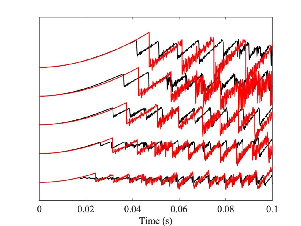
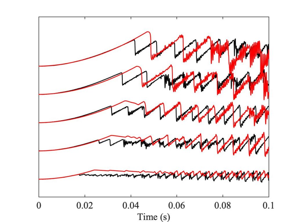
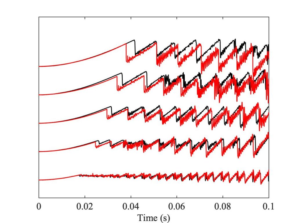
Figure 23 shows that the friction curve model always waits longer than the measurement before the first slip occurs. What then occurs is a jump, even for the lowest bow force at the bottom of the plot. The subsequent details of the waveforms bear very little resemblance to the corresponding measurements. By contrast, Fig. 24 illustrates something we have already anticipated: it never shows an abrupt jump when the rising parabolic shape gives way to the first slip. The bridge force either evolves in a rather flat and featureless way, or for higher values of bow force it shows a rounded hump leading to a gradual jump. The subsequent waveforms do not mimic the measurement very convincingly, although in some cases they do settle quite quickly into a Helmholtz sawtooth shape that echoes the measurement.
Figure 25 shows far more promising behaviour. The first slip mirrors the measurement very well in all 5 cases, which is not a surprise since this first slip information has been used in the development of the model. But, more convincingly in some cases than others, the simulated waveform continues to show something recognisably similar to the measurement across the remainder of the plot. The agreement is by no means perfect, but it is a good deal closer than any of the other cases shown in these plots, and indeed than any previous attempts to model this experiment.
The conclusion is that the enhanced model has taken us a large step closer to reality. First, the effort to formulate this model motivated the new curve fit to the steady sliding measurements shown in Fig. 18, and this has made a big difference to all the Guettler plots. Indeed, the first impression of the collection shown in Fig. 19 is of similarity: all the models now give a recognisable approximation to the pattern shown by the measurements, and in particular the right-hand column shows that both thermal models come quite close to matching the measurement with the real bow. The two thermal models do not, however, predict the same contact temperatures: Fig. 26 shows a comparison, for the final Helmholtz motion from two of the cases shown in Figs. 24 and 25 (the second case from the bottom of each). The original thermal model (in black) predicts a consistently higher temperature than the enhanced model (in red). Both models predict significantly lower peak temperatures than those shown in Fig. 15, based on the original curve fit to the steady-sliding data.
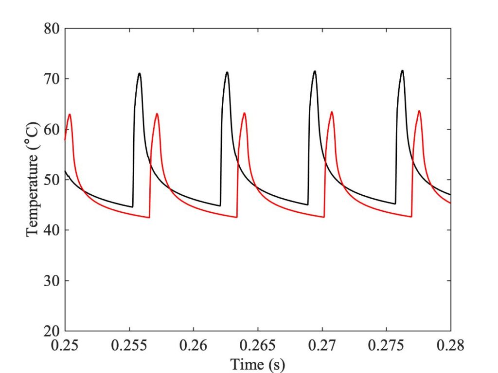
The second improvement shown by the enhanced model is illustrated by Figs. 23—25: in terms of early details of these particular Guettler transients, the enhanced thermal model gives a very creditable match to the measurements; especially when we bear in mind the sensitive dependence of both the real bowed string and the model. We cannot hope to achieve a perfect match to any particular measurement, when we know that any small perturbation to the measurement or to any of the models will change the details.
You may be wondering whether the level of agreement shown in Fig. 25 is a result of “cherry picking” which cases to show. But in fact, a similar level of agreement is seen over the entire Guettler plane. Some more cases, and other details of the comparison between the various models and measurements, are given in the next link. The conclusion from this more thorough survey is tantalising. As we have just seen, the enhanced thermal model gives the best prediction for some aspects of the measurements. But for others, especially with bow positions further from the bridge, the original thermal model seems to do a better job. This leaves a feeling that we are very close to having a universal model, but that we are not quite there yet.
There are still many ways in which the models discussed here do not capture the underlying physics with full accuracy. One of those missing factors concerns the fact that all the simulation models so far have assumed that the bow acts on the string at a single point. But there are important consequences of the finite width of the ribbon of bow hair, and indeed of other aspects of the rather complicated structure of a real bow. Finite bow width will be addressed in the next section, and we will then return to the question of how well our best model matches the complete body of measurements.
[1] J. A. Greenwood and J. B. P. Williamson, “Contact of nominally flat surfaces”, Proceedings of the Royal Society of London, Series A: Mathematical and Physical Sciences, 295, 300-319 (1966)
[2] J. H. Smith and J. Woodhouse, “The tribology of rosin”; Journal of the Mechanics and Physics of Solids 48 1633–1681 (2000).
[3] J. Woodhouse, R. T. Schumacher and S. Garoff, “Reconstruction of bowing point friction force in a bowed string”; Journal of the Acoustical Society of America 108 357–368 (2000).
[4] R.T. Schumacher, S. Garoff and J. Woodhouse, “Probing the physics of slip-stick friction using a bowed string”; Journal of Adhesion 81, 723–750 (2005).
[5] J. Woodhouse, “Bowed string simulation using a thermal friction model”; Acta Acustica united with Acustica 89 355–368 (2003).
[6] P. M. Galluzzo, J. Woodhouse and H. Mansour, “Assessing friction laws for simulating bowed-string motion”; Acta Acustica united with Acustica 103, 1080-1099, (2017). DOI 10.3813/AAA.919136
