
It is useful to understand exactly how a temperature-based friction model can be incorporated into the simulation approach described in section 9.2. This sheds some light on the different behaviour of alternative choices of model. First, a reminder of how the original friction-curve model is dealt with. At each time step, the new values of friction force and string velocity are found by the geometric construction illustrated in Fig. 1, which is a repeat of Fig. 7 from section 9.2.

The history of the string motion allows us to compute the current value of the variable we called $v_h$, and this determines the position of a sloping straight line. We then have to find the intersection of that straight line with the curve representing friction force as a function of velocity, including the vertical segment which represents the range of possible values of force during sticking. Three possible positions of the straight line are shown, and two versions of the friction-velocity curve corresponding to different values of the bow force. For the solid red friction curve, the blue line labelled c indicates an ambiguity, which is resolved by a hysteresis loop involving jumps of force and velocity, as illustrated in Fig. 2 (which is another repeat of an earlier figure).

The original thermal friction model is based on the assumption that the the friction force is proportional to the normal bow force, and that the coefficient of friction is a function $\mu(T)$ of temperature $T$ alone. In order to ensure that the friction force always opposes the direction of sliding motion, the friction force $f$ must then take the form
$$f=-F_b \mu(T) \mathrm{sgn}(v) \tag{1}$$
where $F_b$ is the bow force, and $\mathrm{sgn}(v)$ denotes the sign function, equal to $\pm1$ depending on whether $v$ is positive or negative. What this means for the simulation is that at each time step we first calculate the temperature, and hence obtain $\mu$, then to deal with the $\mathrm{sgn}(v)$ term we solve a version of the graphical construction illustrated in Fig. 3. This function has a vertical portion representing the state of sticking, but during sliding the function is simply constant, so there can be no jumps and no hysteresis loop.

There is another possible temperature-based friction model we could have explored. The measurements on the bulk properties of rosin shown in Fig. 8 of section 9.6 suggest that over most of the relevant temperature range rosin behaves predominantly as a viscous liquid. That would suggest a friction law taking the general form
$$f=-F_b \zeta(T) v . \tag{2}$$
The function $\mathrm{sgn}(v)$ has been replaced by simple proportionality to $v$, because a viscous shear force is proportional to shear rate. This factor $v$ achieves the desired effect of reversing direction according to the sign of the sliding velocity, but it has a very drastic effect on the predicted behaviour. Figure 4 shows the graphical representation equivalent to Figs. 1 and 3. This time, there is no barrier whatever representing “sticking” behaviour. Simulations based on such a model will regularly show “forward slipping”, something that is never (or virtually never) seen in measurements.

A viscous-based model like this is clearly not, therefore, a good candidate for the true friction law. The explanation for this apparent conflict with the measured properties of rosin lies in the particular conditions of those measurements. The rheometer tests used extremely small strains and strain rates, in order to keep the behaviour in the linear range. But the bowed string motion we are interested in involves intervals of gross sliding. This will take the material well outside the range of the rheometer tests.
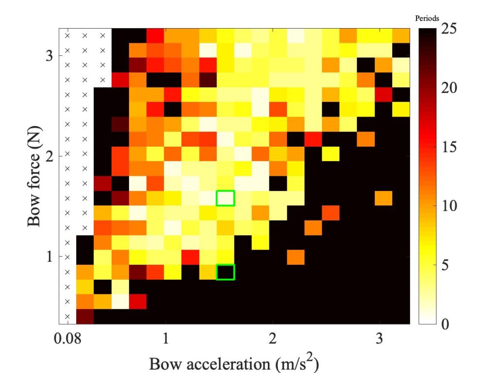
Examples of the measured bridge force for two different constant-acceleration Guettler transients are shown in Fig. 5. Both have the same bow acceleration, but they have different values of the normal force $F_b$. Figure 6 shows the context of these two cases in the Guettler plane. The upper plot in Fig. 5, with the higher value of $F_b$, shows a waveform that settles very quickly into the sawtooth form of Helmholtz motion, while the lower plot shows a rather hesitant start leading to an irregular sawtooth wave of shorter period.
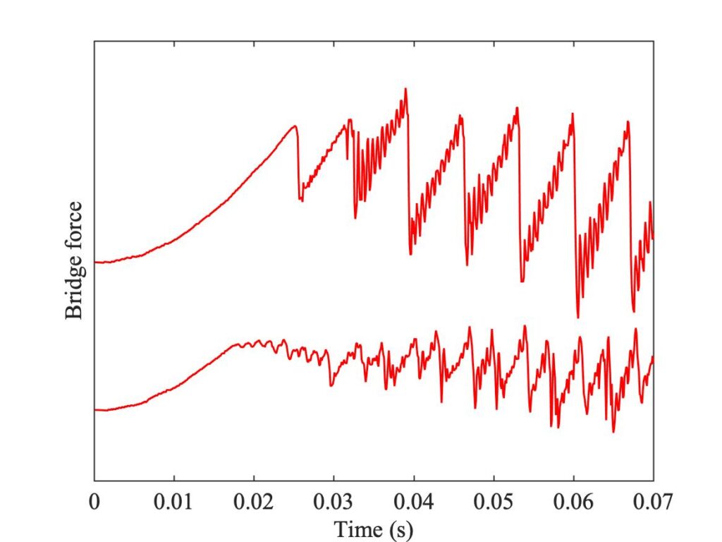
Both bridge force waveforms in Fig. 5 begin with a smooth parabolic rise. During this rise, the string is sticking to the bow-hairs and being pulled sideways in a quasi-static manner. With constant bow acceleration $a_b$, the displacement at the bowed point is given by $y=a_b t^2/2$. A simple static force calculation then says that the friction force at the bow is
$$f \approx \dfrac{Py}{L \beta (1-\beta)} \tag{3}$$
where $P$ is the string tension, $L$ is the string length, and the position of the bow on the string is a distance $\beta L$ from the bridge. The bridge force is
$$f_{br} \approx \dfrac{Py}{\beta L} \tag{4}$$
so that
$$f \approx \dfrac{f_{br}}{1 – \beta} . \tag{5}$$
Equation (3) accounts for the parabolic rise, and equation (5) allows the peak value to be converted to the peak friction force.
After the parabolic rise, the two waveforms in Fig. 5 behave differently: the upper plot shows an abrupt jump, but the lower one does not. Note that eq. (5) only applies during the parabolic rise: a sudden jump in friction force is transmitted to an identical jump in bridge force, without the factor $(1-\beta)$. The case with a jump highlights a major shortcoming with the thermal model described above: as we have already commented, this model is unable to give such an initial jump in friction force, it always behaves more like the lower plot.
We need to modify the original thermal model in some way to allow the possibility of an initial jump in bridge force. There is a very simple, if apparently ad hoc, approach, motivated by Figs. 1 and 2. We can replace the function $\mathrm{sgn}(v)$ in equation (1) by something like the function plotted in Fig. 7. The middle one of the three blue lines shows that this function can exhibit multiple intersections, and therefore sometimes predict jumps and hysteresis. But note that the range of velocity plotted here is much wider than in Fig. 1: the red curve sketched here has a falling shape which is much gentler than the original friction curve.

Figure 7 is just a sketch, using a somewhat arbitrary curve, but we can make use of measurements in the Guettler plane to construct a particular curve that should reproduce an aspect of the true behaviour. In place of equation (1) we can write the friction force in the form
$$f= -A~h(v)~ Y(T) \tag{6}$$
where $h(v)$ is a function of sliding speed generically similar to Fig. 7, $A$ is the area of contact between rod and string, and $Y(T)$ is a yield stress that depends on temperature. This describes a friction curve model in which the friction curve is scaled down as temperature rises, so that jumps by the mechanism of Fig. 2 become less likely. If Coulomb’s law is still to apply, then we require $A$ to be proportional to the bow force $F_b$, so introduce a constant $K$ such that
$$A = K F_b . \tag{7}$$
The pattern of jumps in the measured Guettler data can be used to test whether this idea has any merit, and to give information about the required form of $h(v)$. From a waveform like the upper plot in Fig. 5, values can be determined for the maximum friction coefficient just before the jump, and for the subsequent jump in friction coefficient. If that jump is caused by the phenomenon illustrated in Fig. 2, points can then be plotted in the $\mu -v$ plane representing the two ends of the jump: we know the slope of the straight lines in Fig. 2, and we know that at the start of the jump the relative sliding speed is zero (at least approximately). Repeating the analysis for different cases of the Guettler plane scan, if eq. (3) is to hold and if the temperature is the same in all cases when the jump occurs, $T_0$ say, the points should all fall on a curve $K h(v) Y(T_0)$.
Figure 8 shows the variation across the Guettler plane of the maximum friction coefficient before the first slip. It shows that there is something a little odd about the three leftmost columns: the maximum friction coefficient is far higher than in the rest of the plot. Possibly at these very low accelerations the rosin in the contact region had time to “set”, whereas at the higher accelerations it remained softer? There isn’t enough data to be certain, but we will exclude these columns from the analysis we are about to describe. The remainder of the plot shows a rather uniform colour.
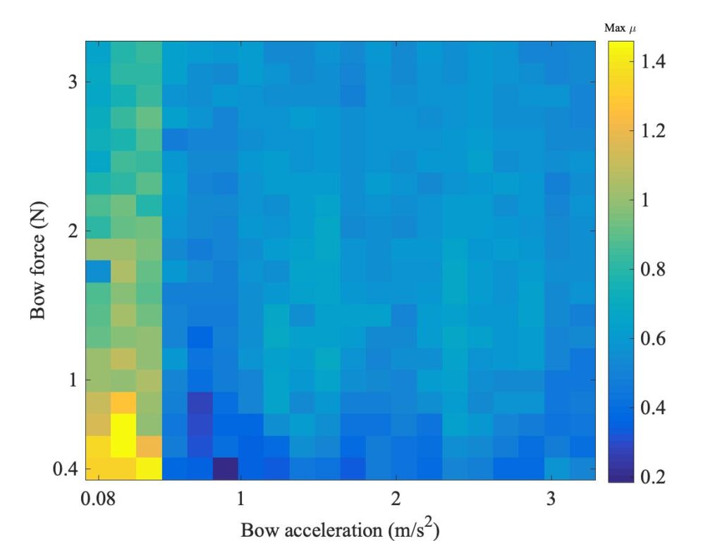
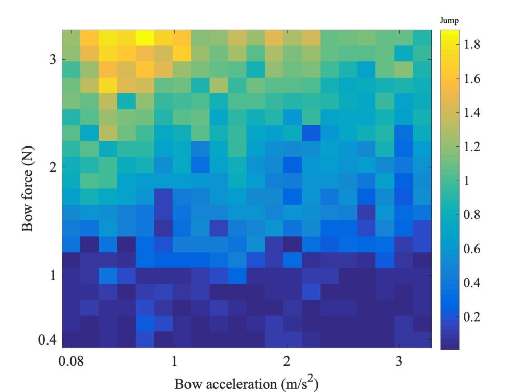
Figure 9 shows the corresponding variation of the magnitude of the initial jump in the Guettler plane. The pattern it reveals it just what we would expect from a model like Fig. 7. The bottom third of the plot shows very dark colours, telling us that for low values of the bow force there was essentially no jump — as the lower plot in Fig. 5 showed. But at higher force, a threshold is crossed and jumps start to occur — small ones at first, then progressively bigger ones as the bow force increases.
Combining this information into a plot in the $\mu – v$ plane gives the cloud of red stars in Fig. 10. To reduce scatter, for each value of acceleration the friction coefficients in the corresponding column of Fig. 8 were averaged. It is immediately clear that these red stars do indeed map out a consistent curve, albeit with some scatter (due in part to the inevitable uncertainty associated with the automated routine used to identify the initial jumps). The black line is a fit to this curve, which will be explained in detail shortly.
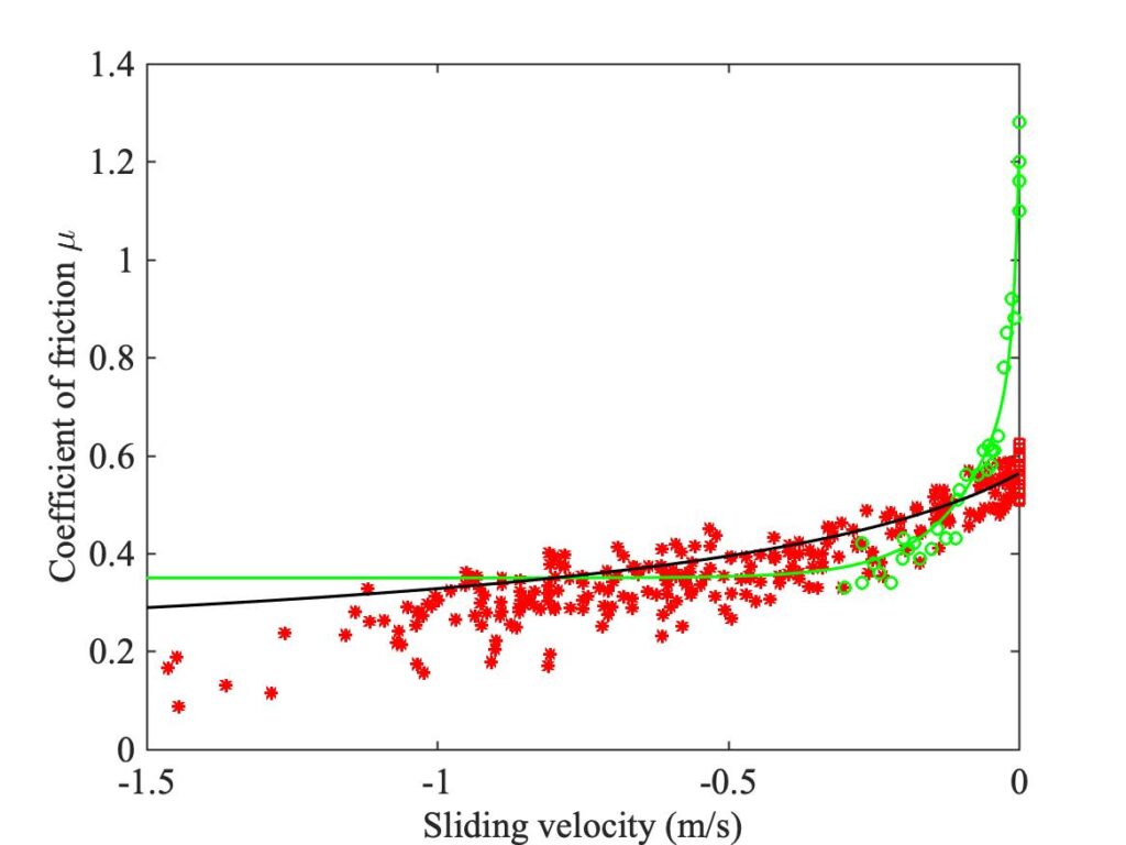
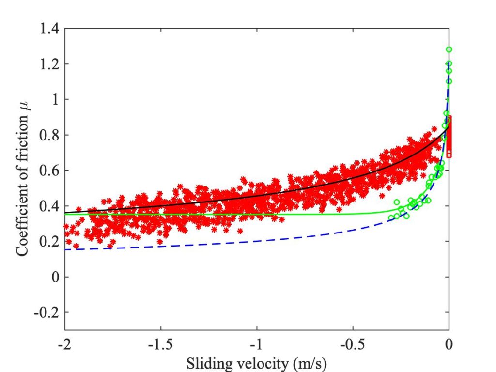
Figure 11 shows the result of applying the same analysis to Guettler scan data obtained using a normal cello bow in place of the rosin-coated rod. This time, data from 4 different bow positions $\beta$ has been combined so that there are more red stars than in Fig. 10. This cloud of stars again maps out a consistent curve, if anything rather more clearly than for the rod case in Fig. 10.
As in the original thermal model, the temperature-dependent function $Y(T)$ from equation (6) can be determined by requiring that the new model should reproduce the measured results under conditions of steady sliding. Since $h(v)$ and $Y(T)$ appear as a product, there is an undetermined factor that could multiply one while dividing the other. It is convenient to fix this factor by requiring that the curve fitted to the red stars, $\mu_{jump}(v)$ say, is simply equal to $h(v)$. This requires
$$K Y(T_0) = 1 \tag{8}$$
in terms of the constant $K=A/F_b$ introduced earlier. For steady sliding, we then require
$$\mu_{steady}(v) = K h(v) Y(T_{steady}(v)) = h(v) Y(T_{steady}(v))/Y(T_0) \tag{9}$$
where $\mu_{steady}(v)$ is the curve fit to the steady sliding data, and $T_{steady}(v)$ is the temperature that results from solving the original heat-balance equation (from ref. [1]) with $\mu(v) = \mu_{steady}(v)$.
For self-consistency of this model, $T_{steady}$ should be a monotonically decreasing function of $|v|$. It follows that
$$\mu_{steady} \gtrless \mu_{jump} \mathrm{~~when~~} T_{steady} \lessgtr T_0 \tag{10}$$
so that $T_0$ is defined by the crossing of the lines representing the two curve fits.
There are now two good reasons why the original curve fit to the steady sliding results, shown by the green line in Figs. 10 and 11, is not a good choice. First, based on the expected material properties of rosin above the glass transition temperature, one would expect $\mu_{steady}(v) \rightarrow 0$ as $v \rightarrow\infty$ because $Y(T)$ will decrease to very small values. Second, by the highest sliding speed shown in Fig. 10 the green curve has risen above the cloud of red stars so that it does not satisfy the inequality (10).
The challenge, then, is to find satisfactory curve fits to both sets of data such that the steady sliding fit leads to a monotonic increase of temperature with sliding speed, and (10) is satisfied. With the parameter values used in the bowing model, it turns out that $T$ is approximately proportional to $\mu_{steady}~\sqrt{|v|}$. In order that $T$ is always increasing with $|v|$, $\mu_{steady}(v)$ must therefore decrease slower than $|v|^{-1/2}$.
The combination of these constraints leaves very little flexibility, but it is possible to find curve fits that satisfy them all. One example of such fits is shown in the black line and the blue dashed line in Fig. 11: they both use a power-law variation $|v|^{-0.4}$ to satisfy the constraint on monotonically increasing temperature for steady sliding. It fits the measured points just as well as the earlier curve, but Fig. 11 shows that it follows a very different trend at higher sliding speeds. This blue dashed line is the function
$$\mu_{steady}(v) = -0.2~\mathrm{sgn}(v)~(|v|+0.011)^{-0.4} \tag{11}$$
while the black line is the function
$$\mu_{jump}(v) = h(v) = -0.5~\mathrm{sgn}(v)~(|v|+0.27)^{-0.4} . \tag{12}$$
Using these expressions, the crossing temperature $T_0$ is $26.2^\circ$ above ambient, or $46.2^\circ$C.
The black line in Fig. 10 shows the fit based on the bowing tests with a rosin-coated rod rather than a normal bow. The curve marked by the cloud of red stars lies at lower values than in Fig. 11. It is still possible to achieve a fit of sorts that satisfies all the constraints using a very similar function, with the same power-law decay with speed and a crossing point with the dashed blue line at a point corresponding to temperature $36.8^\circ$ above ambient, or $56.8^\circ$C. The fit shown by the black line represents the function
$$\mu_{jump}(v) = h(v) = -0.37~\mathrm{sgn}(v)~(|v|+0.35)^{-0.4} . \tag{13}$$
[1] J. H. Smith and J. Woodhouse, “The tribology of rosin”; Journal of the Mechanics and Physics of Solids 48 1633–1681 (2000).