
In order to assess how well the two thermal models can do in predicting bowed-string transients, there are many details we can compare with simulations, and many parameters in the models to explore. This section consists mainly of a gallery of images to illustrate some of the effects. At the end of the section there is a little more detail about the simulation methods, including a list of the main parameter values used.
The first step is to choose a datum case, with which the effect of parameter variations will be compared. The chosen case is similar to the one used to generate Fig. 19 of section 9.6, but with one small modification. In section 9.6 we were making a 3-way comparison between the two thermal models and the original friction-curve model. In order to provide a level playing field for comparing these three, a particular choice was made about contact footprint size. In the friction-curve model, the coefficient of friction fitted to the steady sliding measurements was used directly. But the two thermal models are based on a yield stress, so that the friction force is proportional to the contact area. All three models have so far assumed Coulomb’s law, so for the thermal models the contact area was scaled in proportion to the normal load. If the effective coefficient of friction for steady sliding is to match the experiments, the ratio of contact area to normal force needs to be the same for both experiments.
That is the assumption that was made for the results shown in section 9.6. However, the contact geometry for the steady sliding test was significantly different from the bowing tests, either with the rod or the real bow, and there seems to be no reason to assume that this ratio should have exactly the same value. After a little exploration, it was found that a somewhat different value of the ratio gave a slightly better match to the measured Guettler plots, and this value has been chosen for the datum. Details will be given at the end of the section.
A. Different values of bow position $\beta$
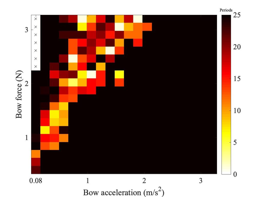
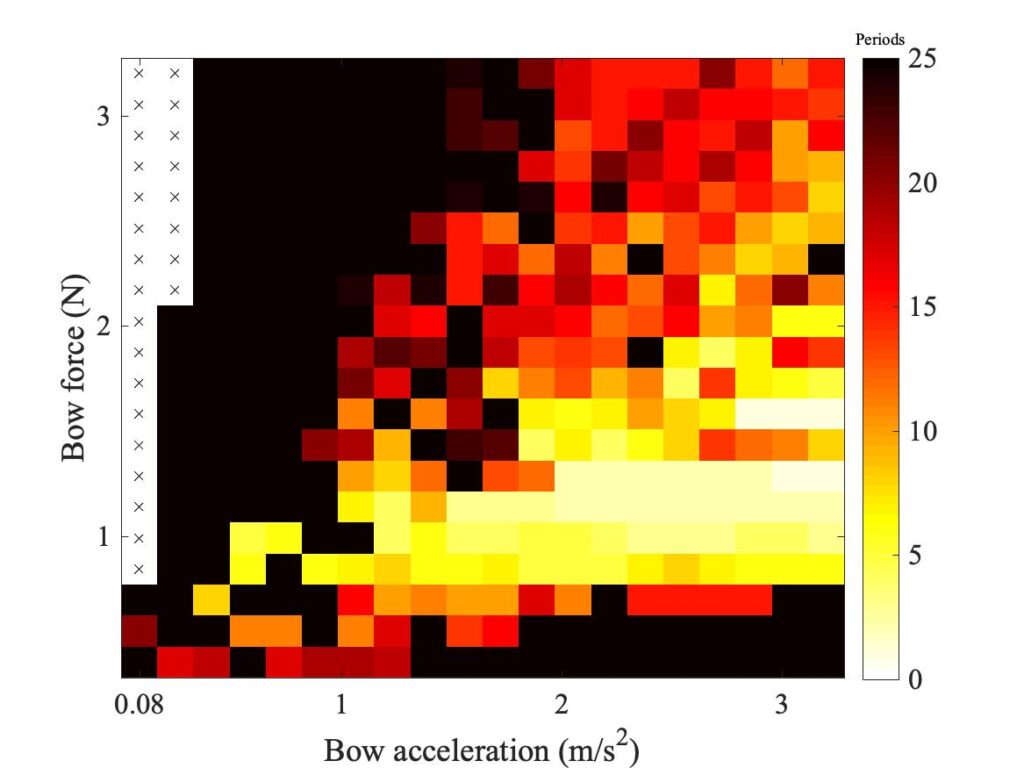
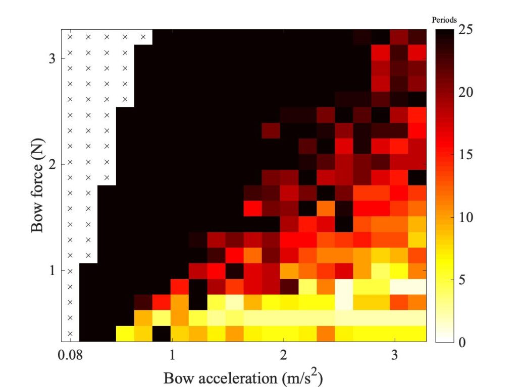
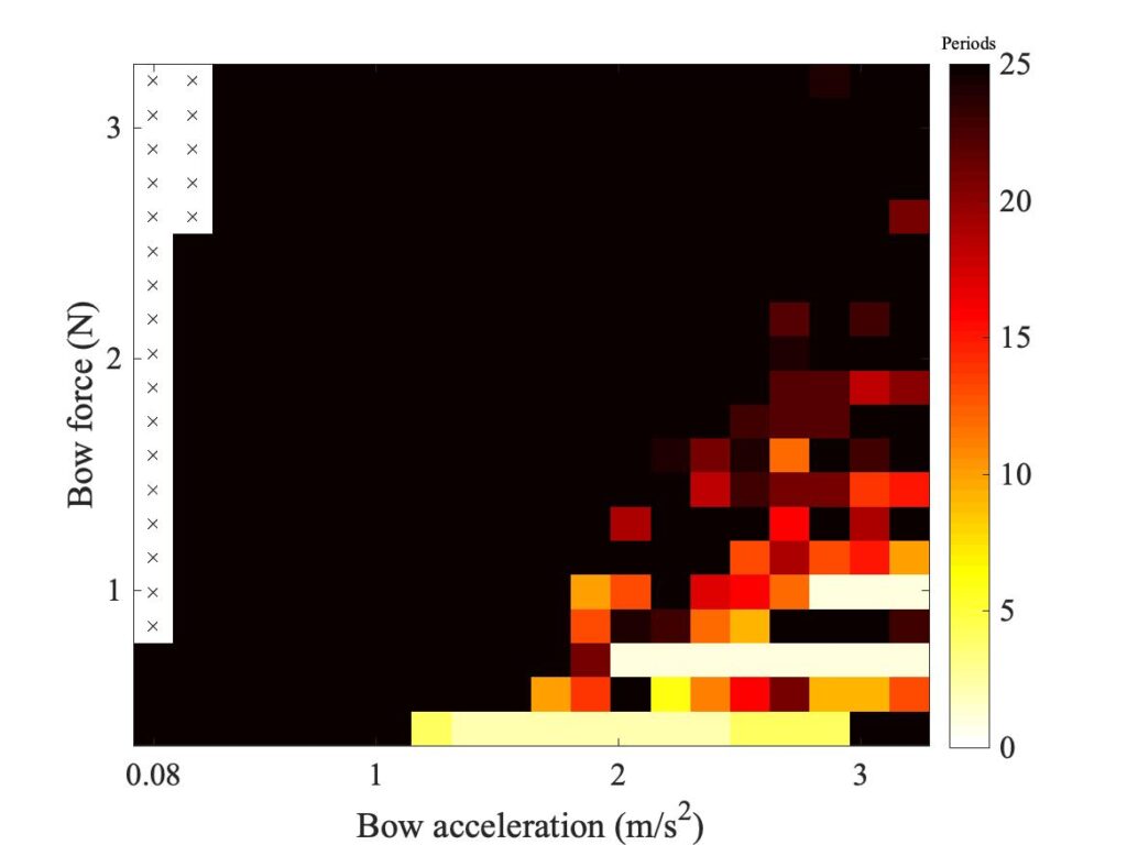
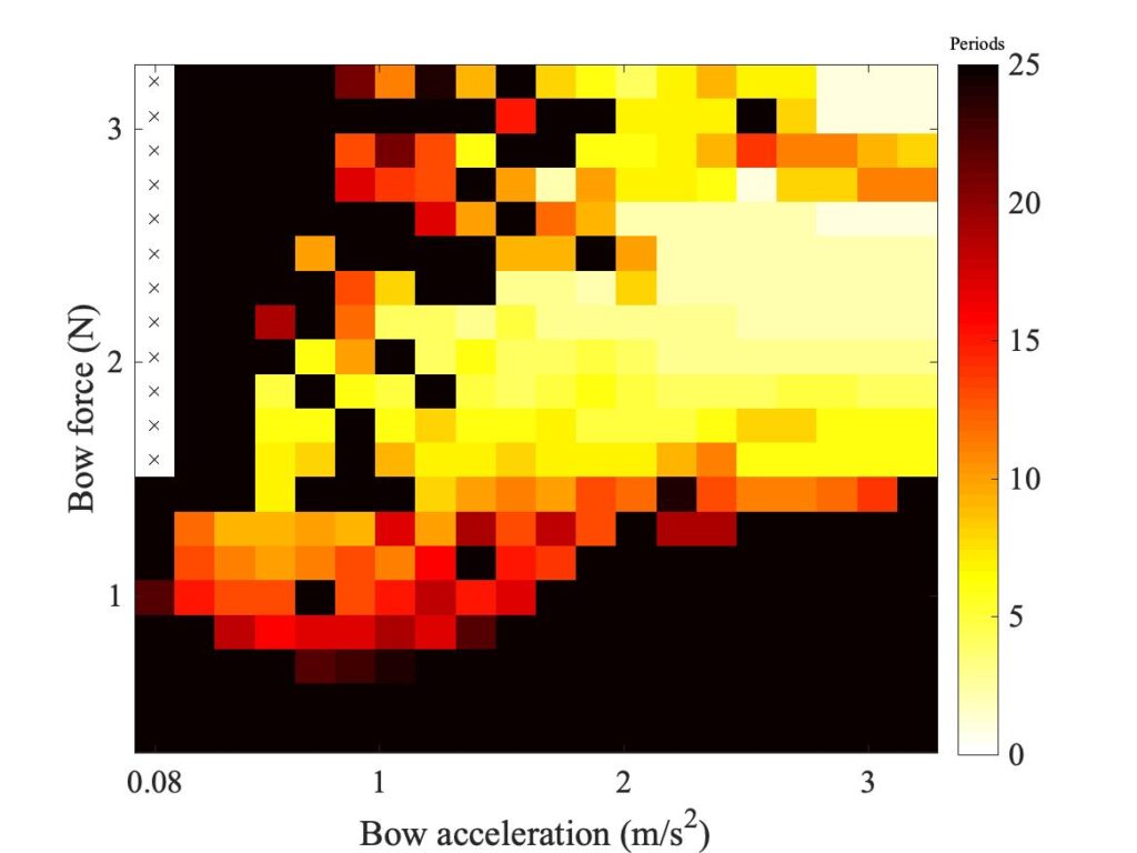
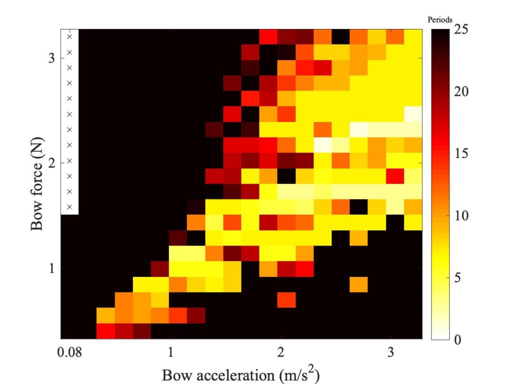
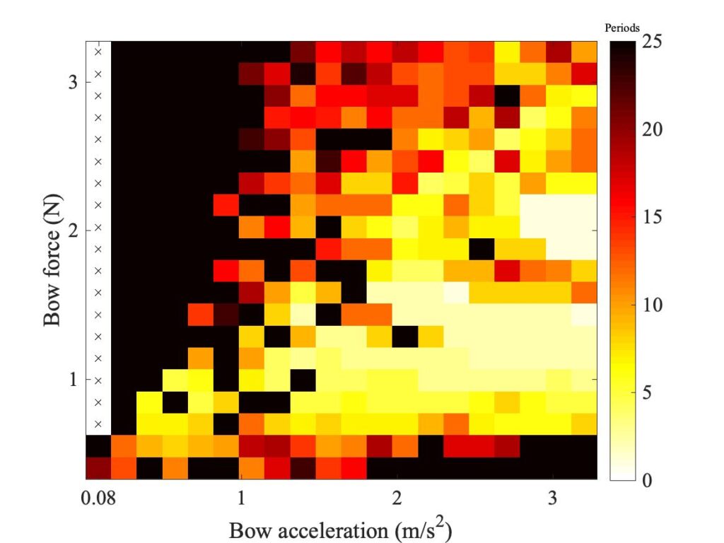
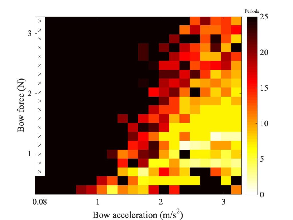
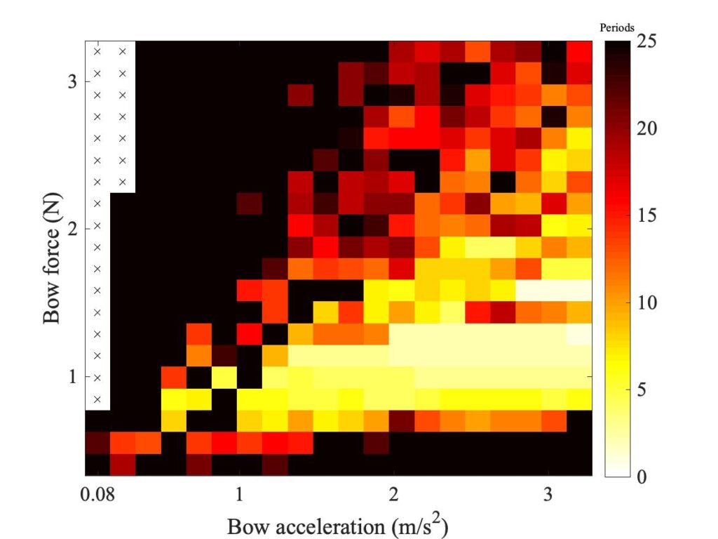
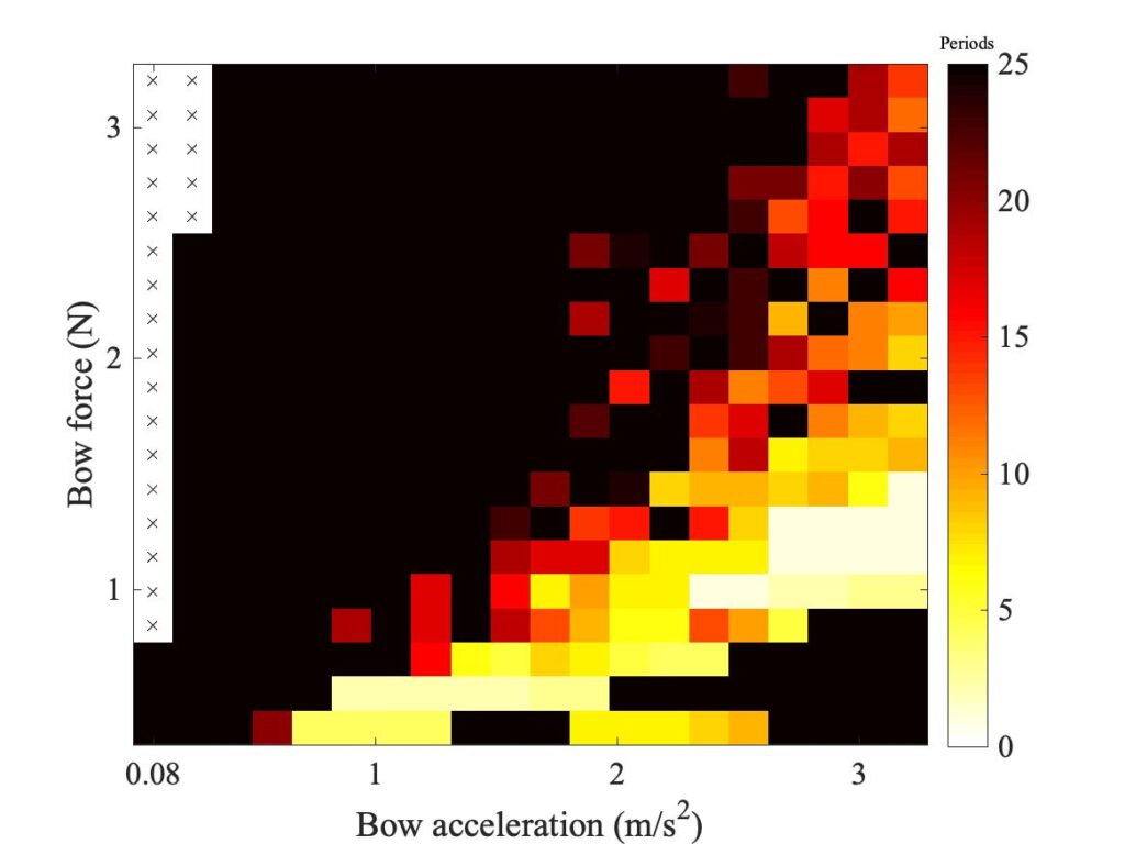
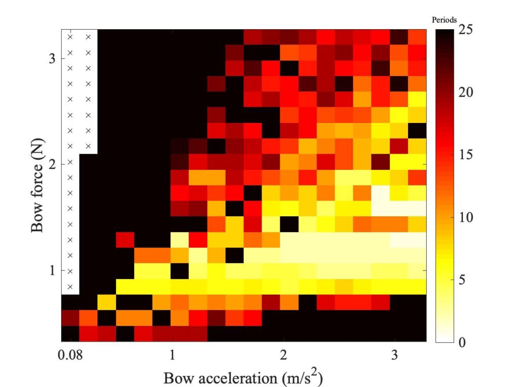
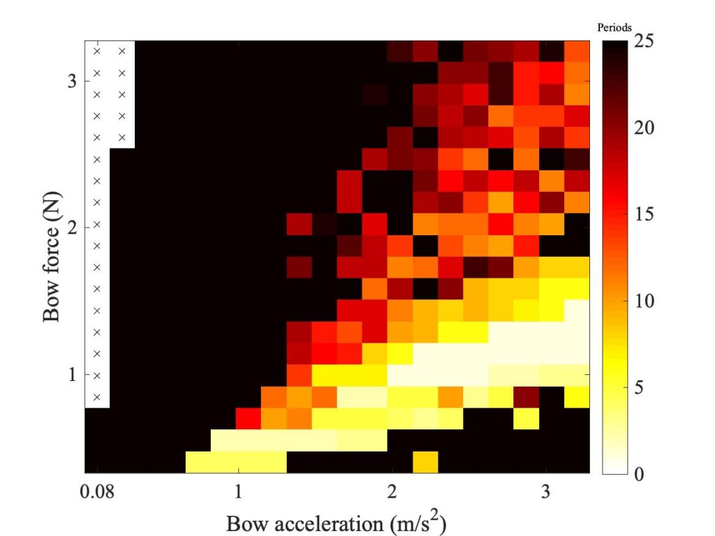
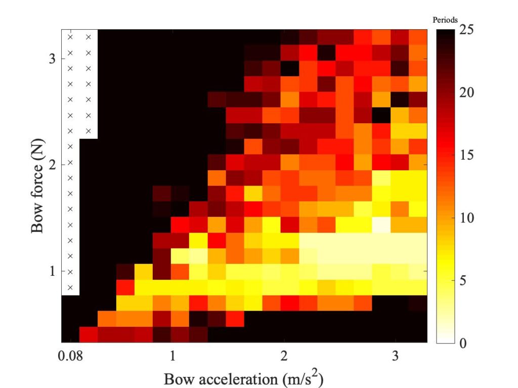
In section 9.6, Guettler diagrams and other results were shown for a single bow position $\beta$, but the measurements and simulations have been carried out for a wide range of $\beta$ values, and some results are shown in Figs. 1—8. Each figure shows four Guettler diagrams. The measured results with the rod and the bow appear in the top row, while in the second row there are simulation results for the datum case, using the original thermal model (left-hand plot) and the enhanced thermal model (right-hand plot). The results shown earlier correspond to the $\beta$ value in Fig. 5.
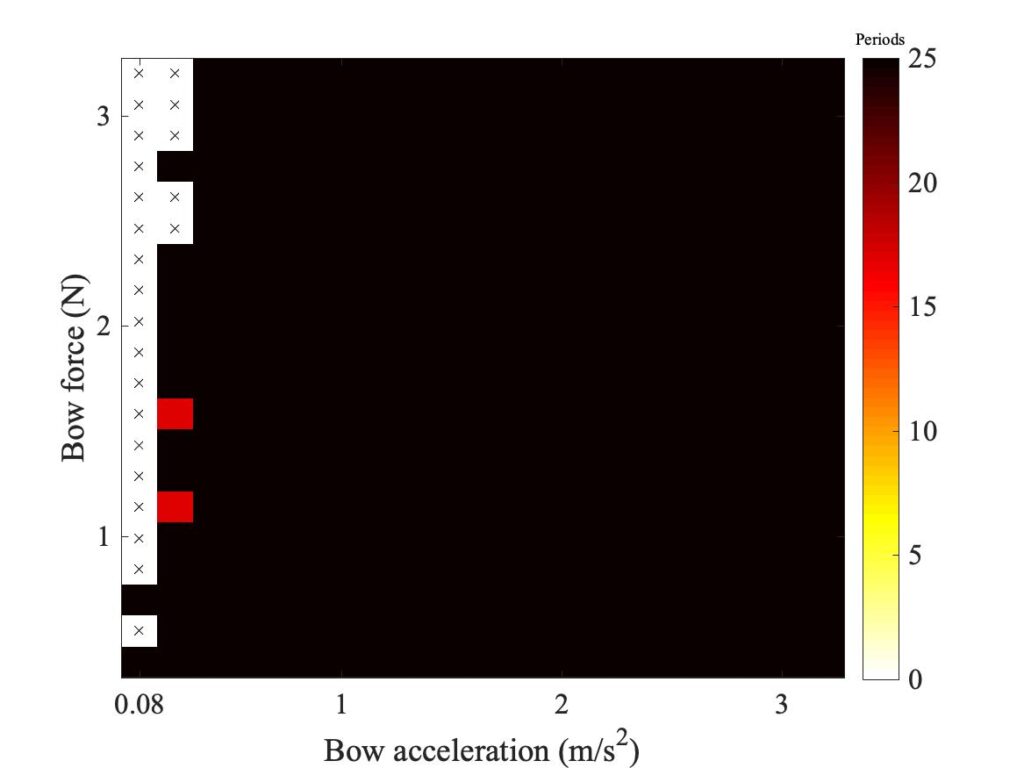
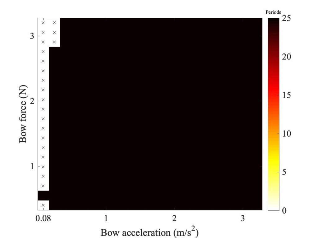
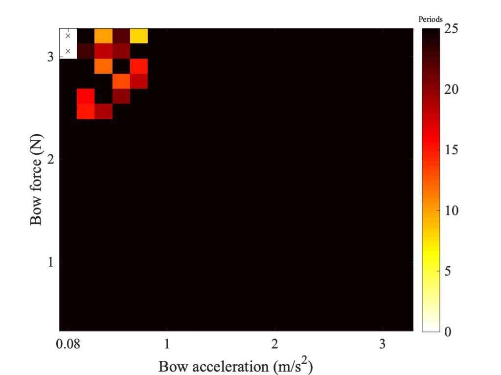
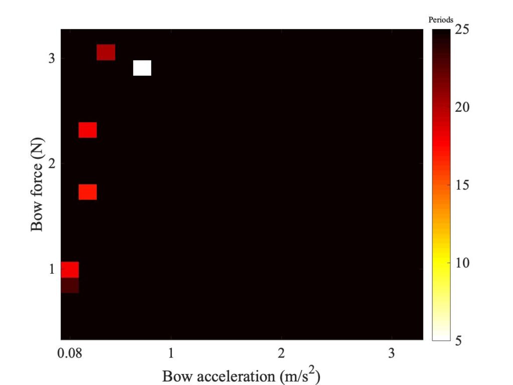
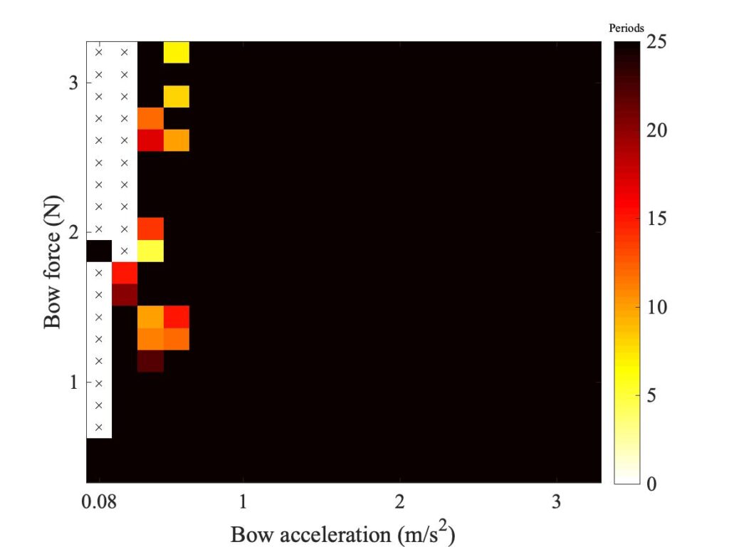
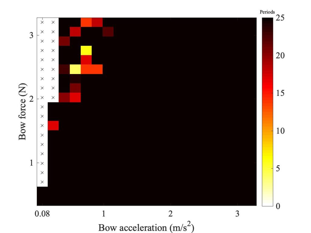
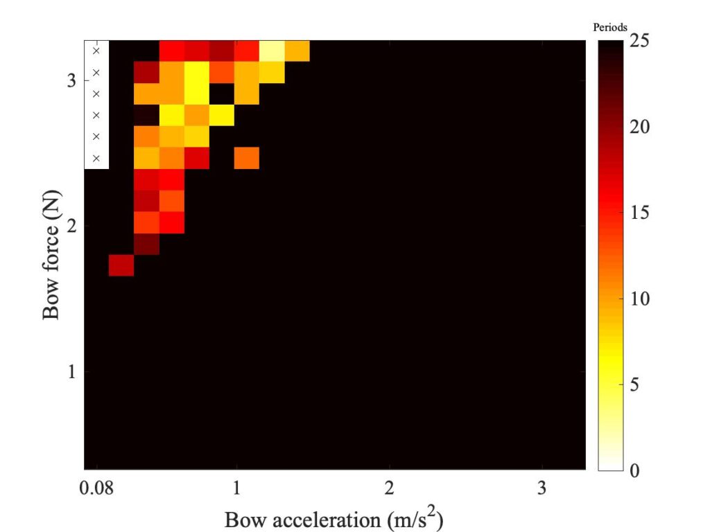
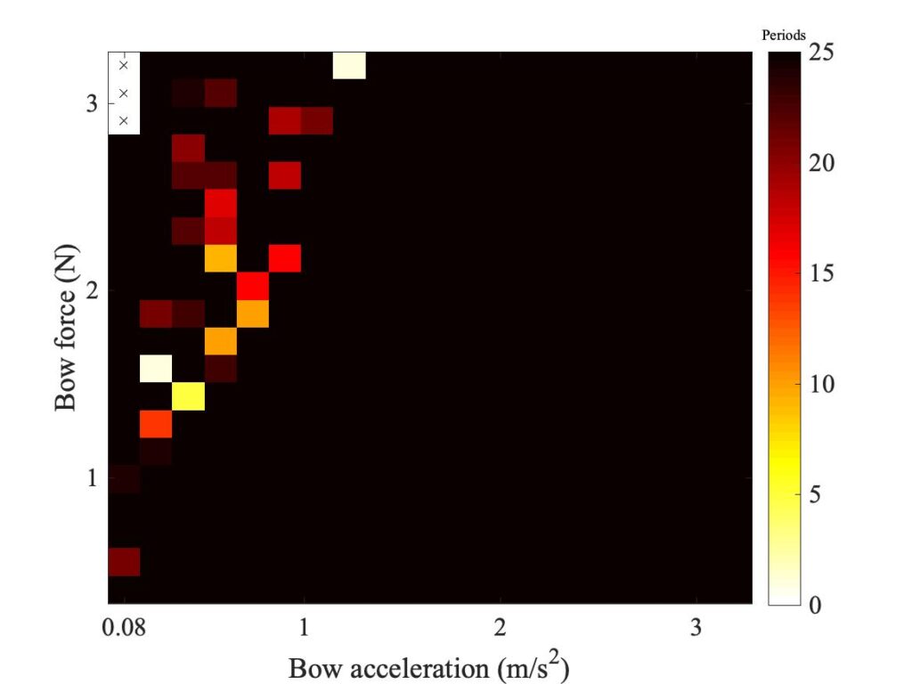
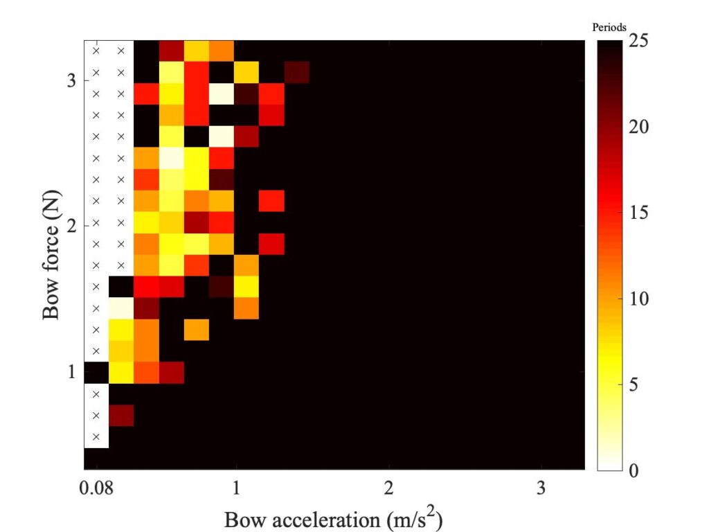
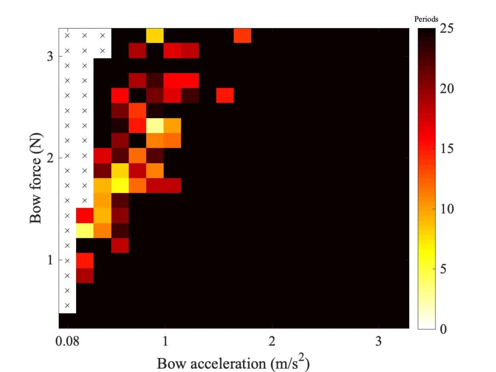
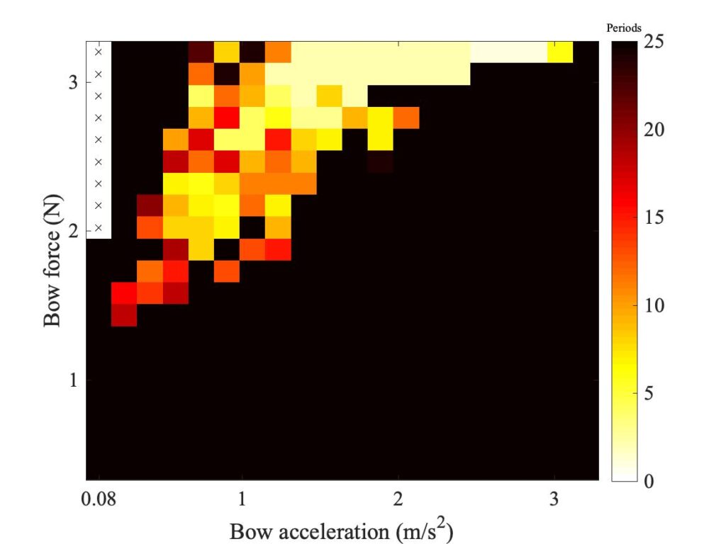
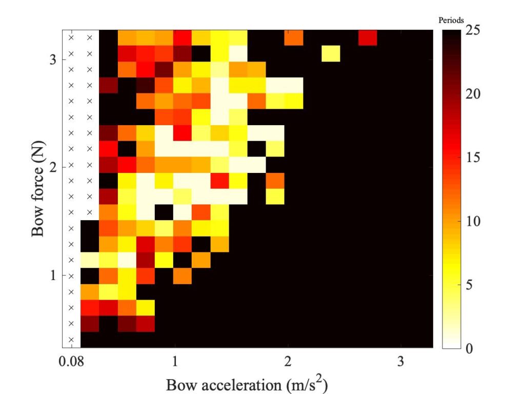
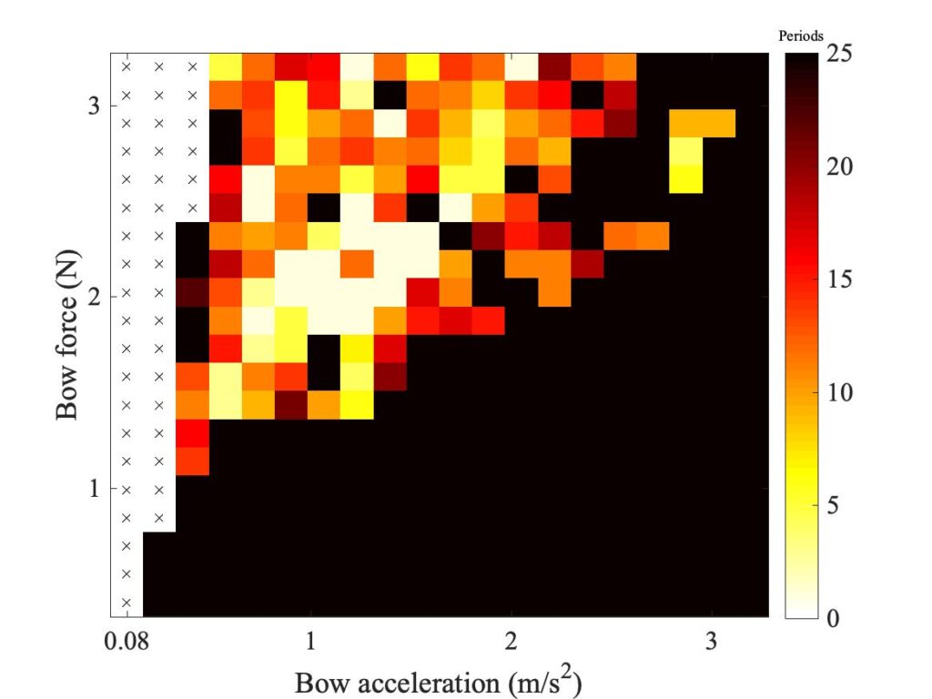
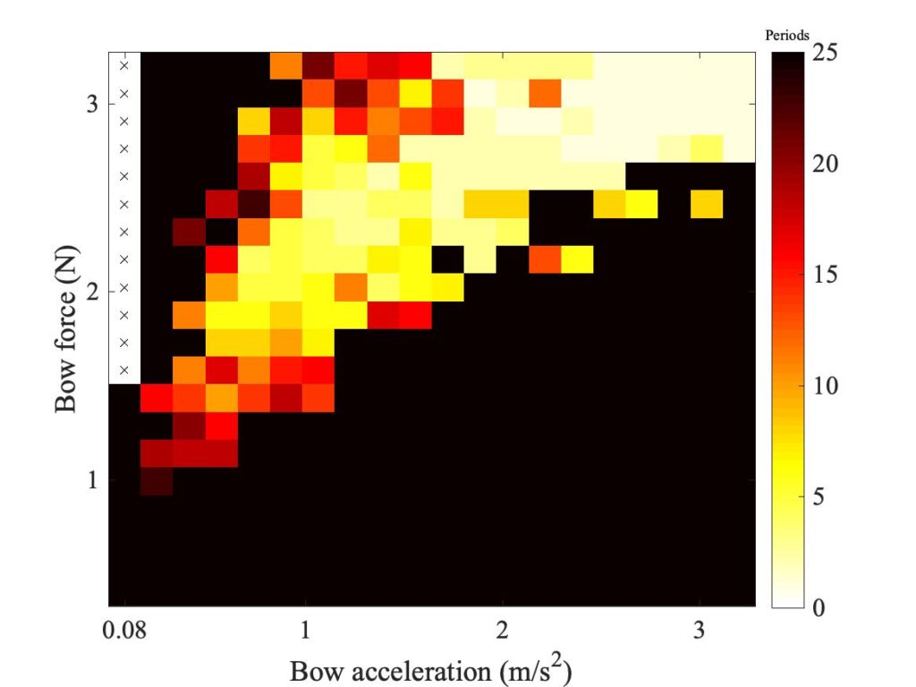
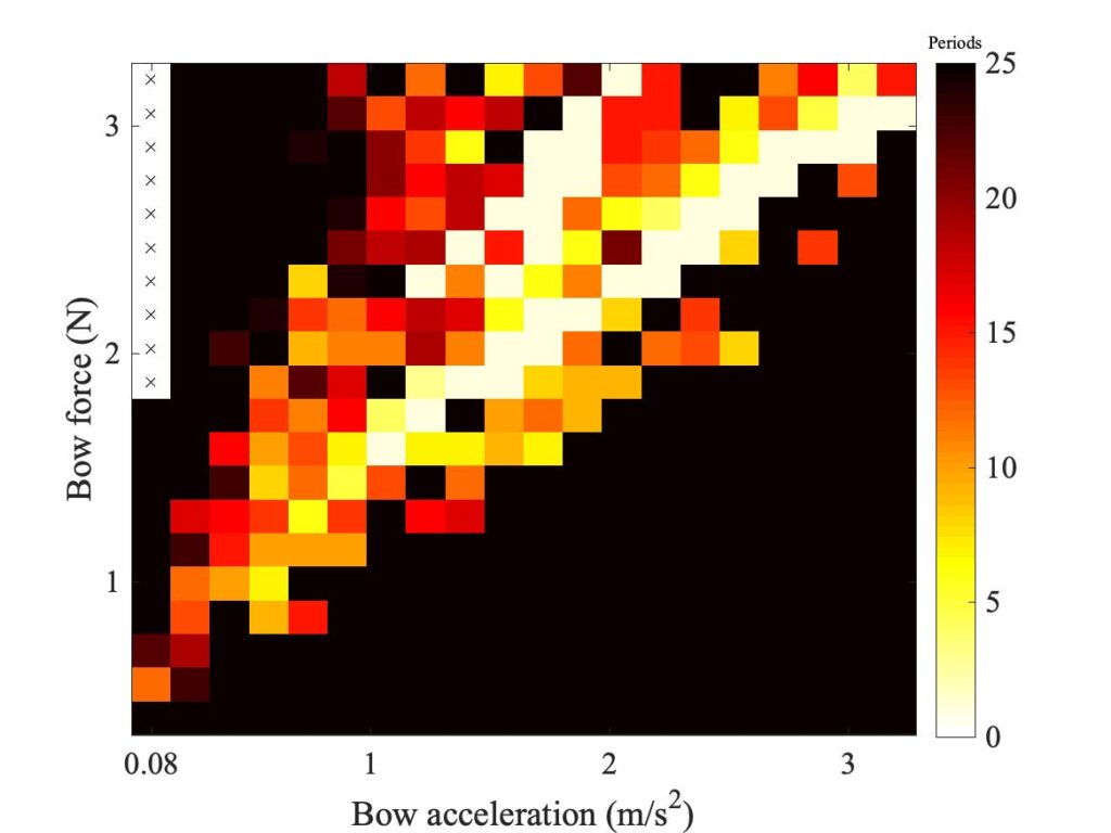
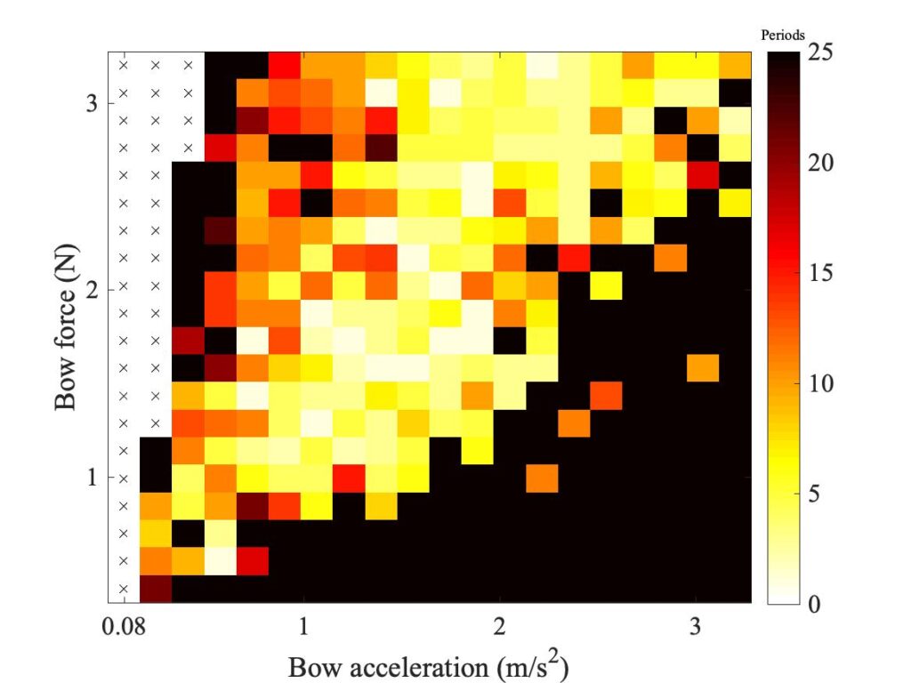
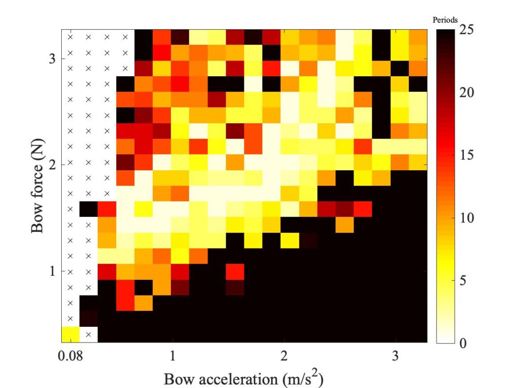
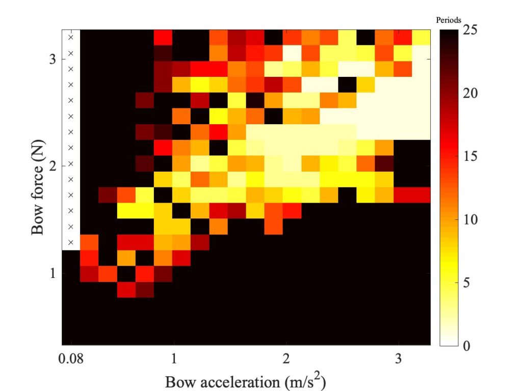
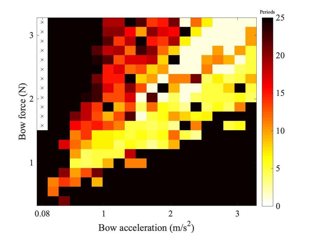
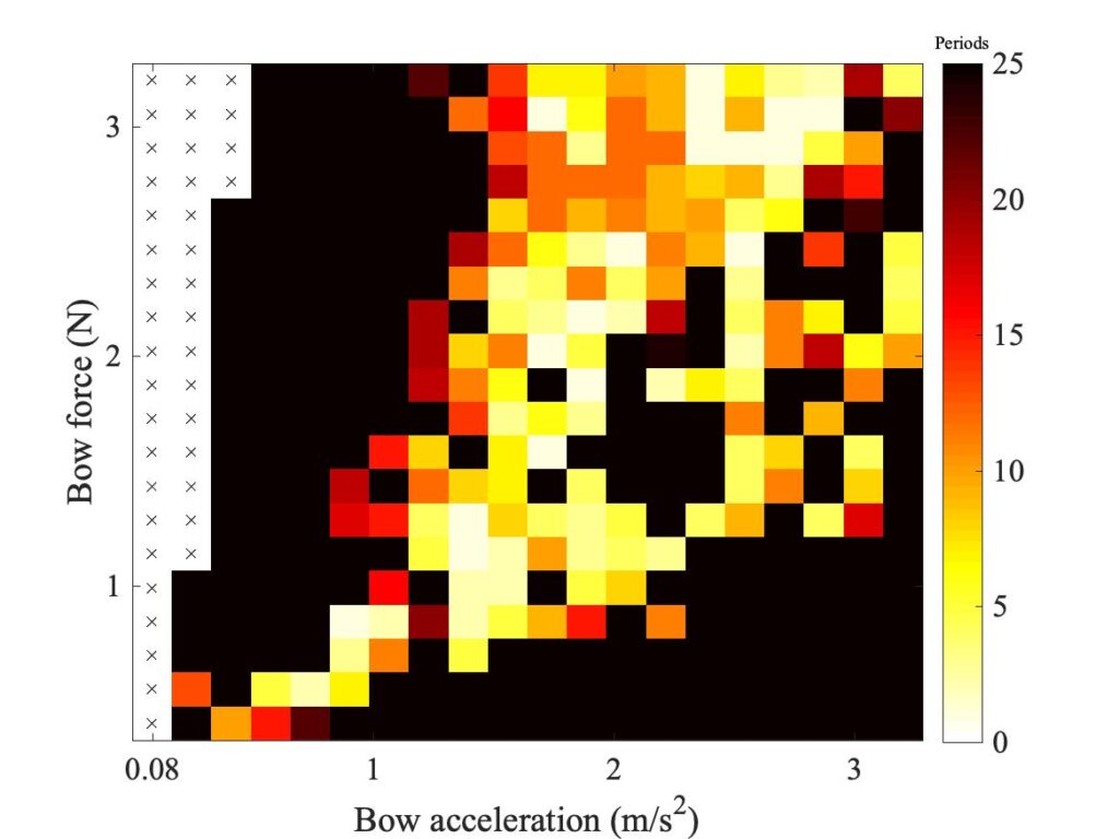
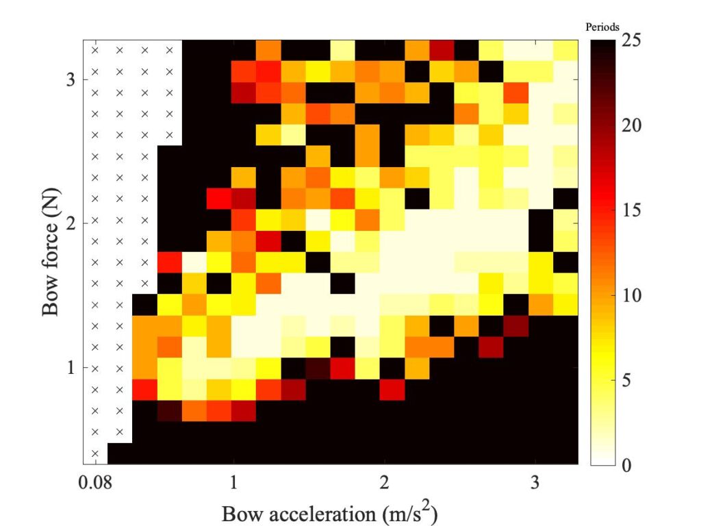
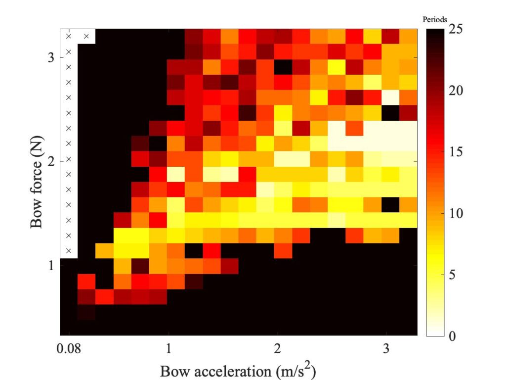
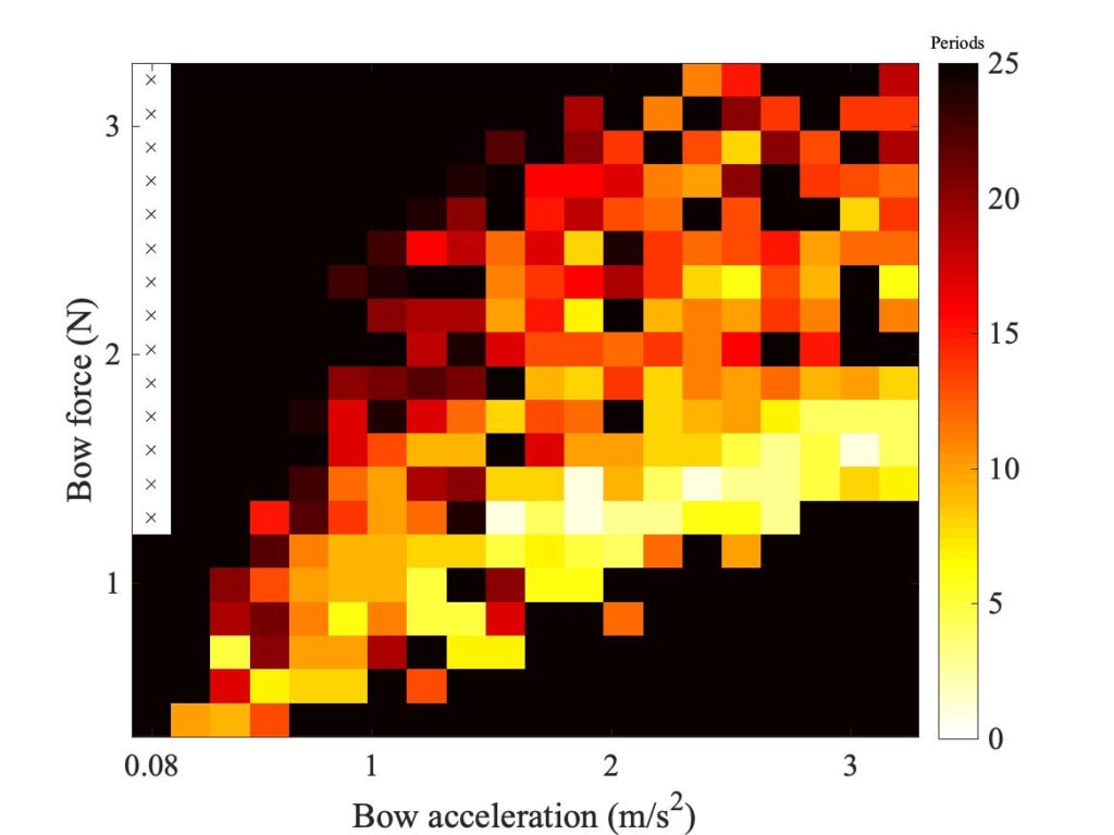
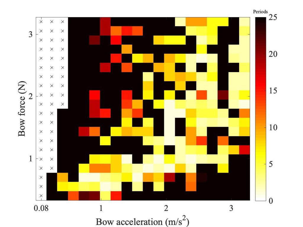
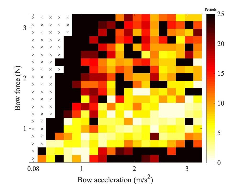
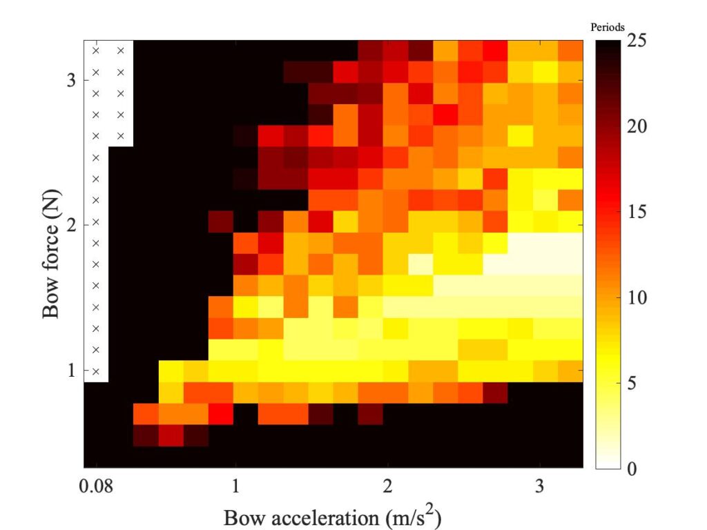
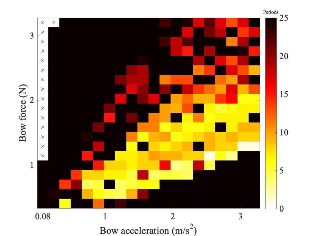
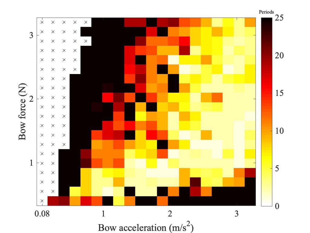

Both simulation models mirror the broad pattern of variation as $\beta$ varies. For low values of $\beta$ (i.e. bowing very close to the bridge), there are very few successful transients. As $\beta$ increases, the region of coloured pixels grows larger and both edges rotate clockwise in the Guettler plane, just as Guettler predicted [1]. If you compare the two plots in the right-hand column in each case (the measurement with the real bow and the simulation with the enhanced model), reasonable agreement is shown in Figs. 1—5, but for the larger values of $\beta$ there is a systematic tendency for the coloured pixels from the simulation to be confined to the lower part of the region where they are seen in the measurement.
The simulations with the original thermal model (bottom left plot in each case) show somewhat less good agreement with the measurements at low values of $\beta$, but in Figs. 6, 7 and 8 they show progressively better agreement, filling in some of the black space in the upper left of the Guettler diagram compared to the enhanced model. By Fig. 8, the original model shows a rather convincing match to the measured case, whereas the “enhanced” model is clearly less good.
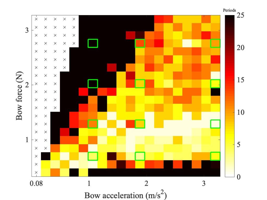
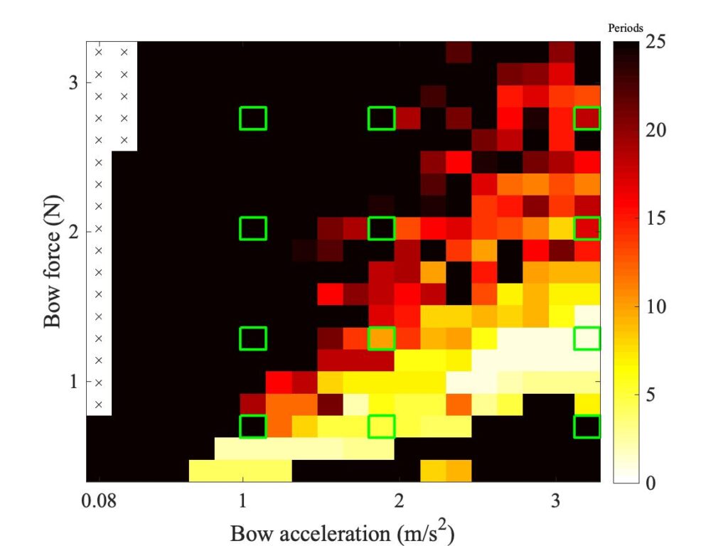
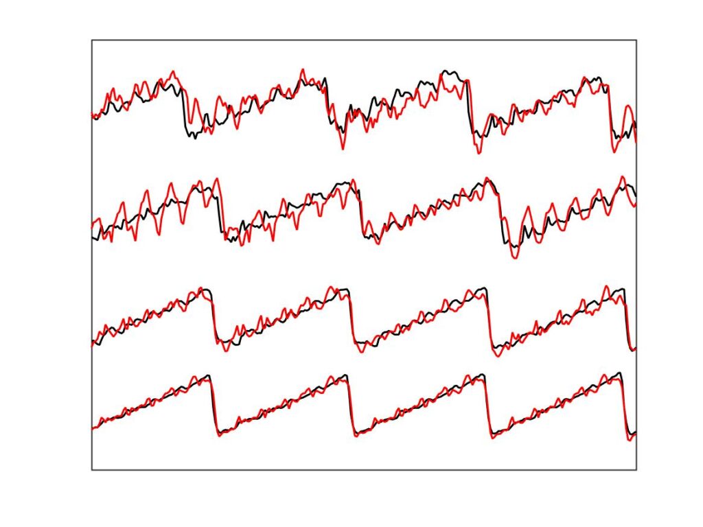
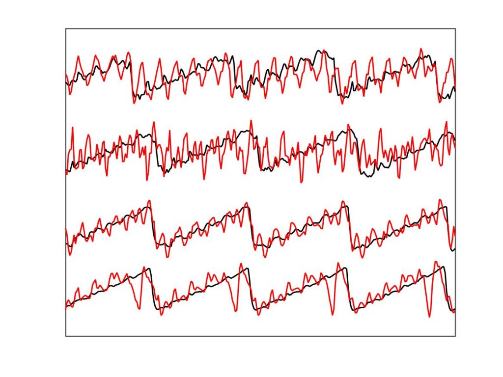
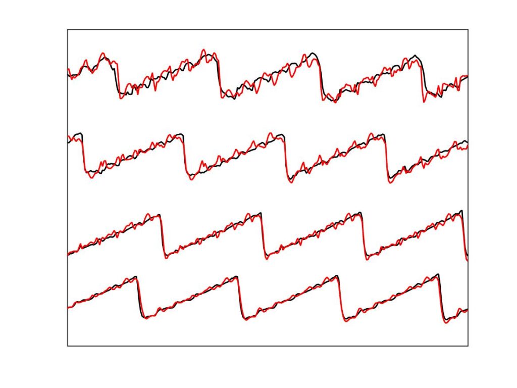
To demonstrate a sense in which the revised model is enhanced, we need to compare the models with a different aspect of the measurements, the early behaviour soon after the first slip. In Fig. 8, a number of cases spread over the Guettler plane are highlighted by green squares. The measured bridge forces for these 12 cases are compared with results from the two thermal simulation models, in Figs. 9, 10 and 11. The results show that the enhanced model (right-hand plot in each figure) gives a pretty good match to all cases, whereas the original model in the left-hand plot always does something quite different at this early stage.
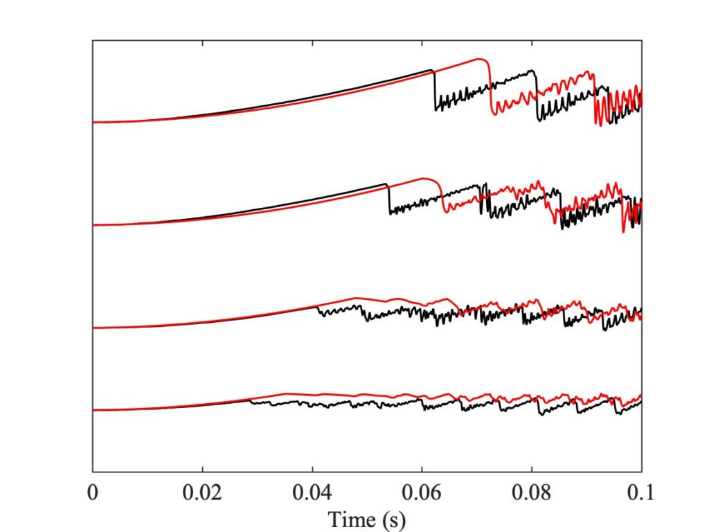
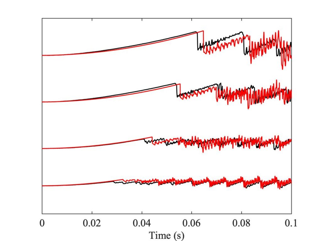
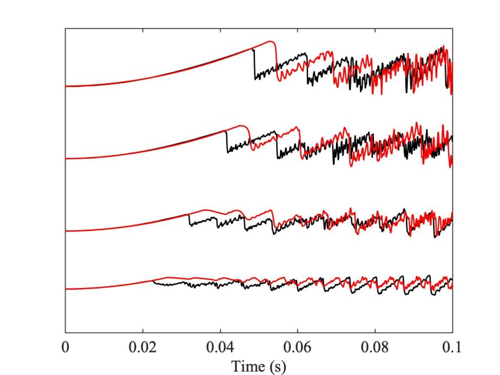
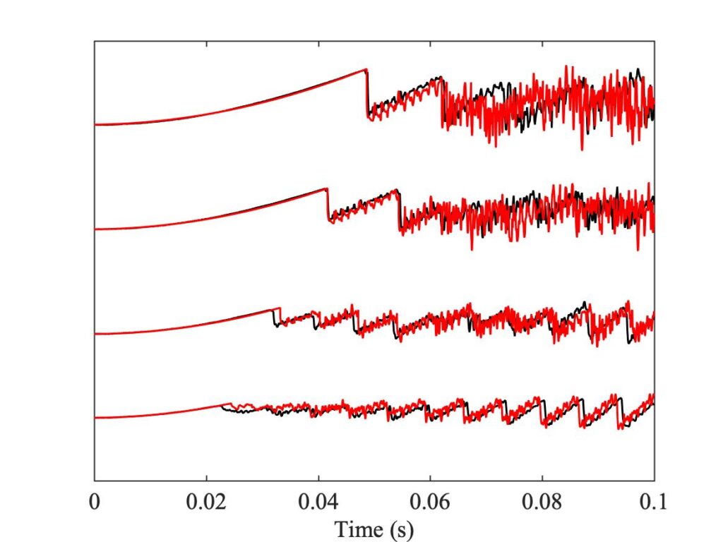
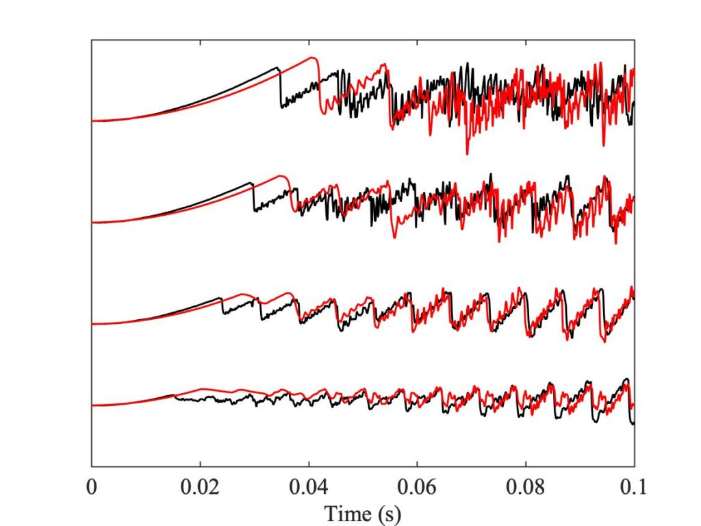
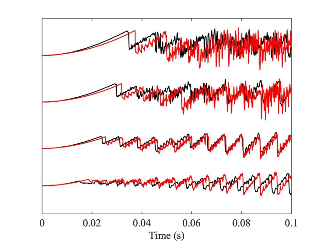
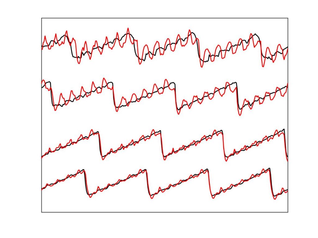
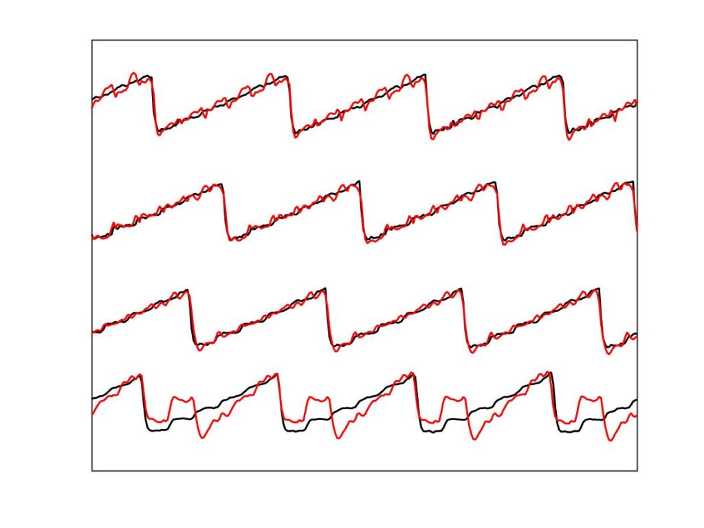
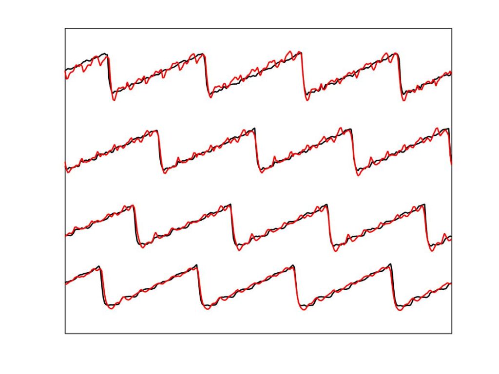
However, we get a different picture when we compare the bridge-force waveforms for these same 12 cases at the end of the measurement period, after 0.25 s. Figures 12, 13 and 14 show the results, with the same layout as Figs. 9, 10 and 11 respectively. These plots show what lies behind the differences in the Guettler plots of Fig. 8. Nearly all cases shown in these plots show some trace of the “Helmholtz sawtooth”, but there is a widespread tendency, especially for the enhanced model, to show bigger “Schelleng ripples” than the measurement. In some cases these ripples grow so large that the automated classification routine has decided that they show “S-motion” rather than Helmholtz motion — particularly in the right-hand plot of Fig. 12, which corresponds to the upper left region of the Guettler diagram where we have already commented that the enhanced model differs most from the measurements.
The conclusion is that neither thermal model on its own can reproduce all details of the measurements, but that any particular aspect of the measurements can be matched by one or other of them. This is a tantalising state of affairs: it feels as if we are quite close to having a satisfactory predictive model. We will resume this discussion in section 9.7, with more detail in section 9.7.2, when we extend the models to allow for the finite width of the bow.
Meanwhile, we have seen that the two point-bow thermal models can do a pretty good job of matching the measurements. This is sufficiently encouraging that it is worth taking a look at the effects on one particular Guettler diagram of deliberate variations in the main parameters of the model. Predictions of both thermal models will be shown side by side, so that there is a good chance that the main effects of these parametric variations will be correctly predicted.
B. Parameter variations
The case to be considered is the one we have just looked at in some detail: the $\beta$ value corresponding to Fig. 8. For convenience, the Guettler diagrams from the two models for this case are reproduced in Fig. 15. As in earlier figures, the original thermal model is shown on the left, and the enhanced model on the right. All subsequent plots will have this same layout.

The first group of parameters to be explored concern the frictional contact between bow and string: the contact area and shape, and the thickness of the actively deforming rosin layer. These are the parameters whose values are most in doubt: it is very hard to get direct empirical information about any of them. Figure 16 shows the effect of changing the assumed area of contact between “bow” and string. In the top row, that area has been doubled; in the bottom row it has been halved. This reveals a general trend that is the same for both models: increasing the area of contact shifts the region of coloured pixels downwards, while decreasing the area shifts the region upwards.
So far, all the simulations have assumed a circular contact footprint, as in the original description of the thermal model [2]. But the actual contact geometry in the measurements will surely not be circular. With the rod it might be expected to be an elliptical area, narrower in the sliding direction and wider in the perpendicular direction. With the real bow, there will be a large number of separate contact areas, between individual bowhairs and the string. The combined effect of these will probably be a more extreme version of the same pattern, narrow in the sliding direction and wider in the perpendicular direction. In the next subsection, a very simple extension of the model from [2] will be described, to allow an elliptical footprint.
Figure 17 shows some examples of the effect. In the top row, the contact footprint is an ellipse of the same total area as the datum case, with aspect ratio 3:1. In the bottom row the ellipse has the more extreme aspect ratio 9:1. The plots in the top row are not very different from the datum case in Fig. 15. The bottom row shows a slightly bigger effect, with the region of coloured pixels shifted slightly downwards for both models. However, the effect seems small compared to the sensitivity to contact area shown in Fig. 16, and indeed one would guess that this drastic departure from circularity of the footprint could be compensated by a small decrease in the total area of contact.
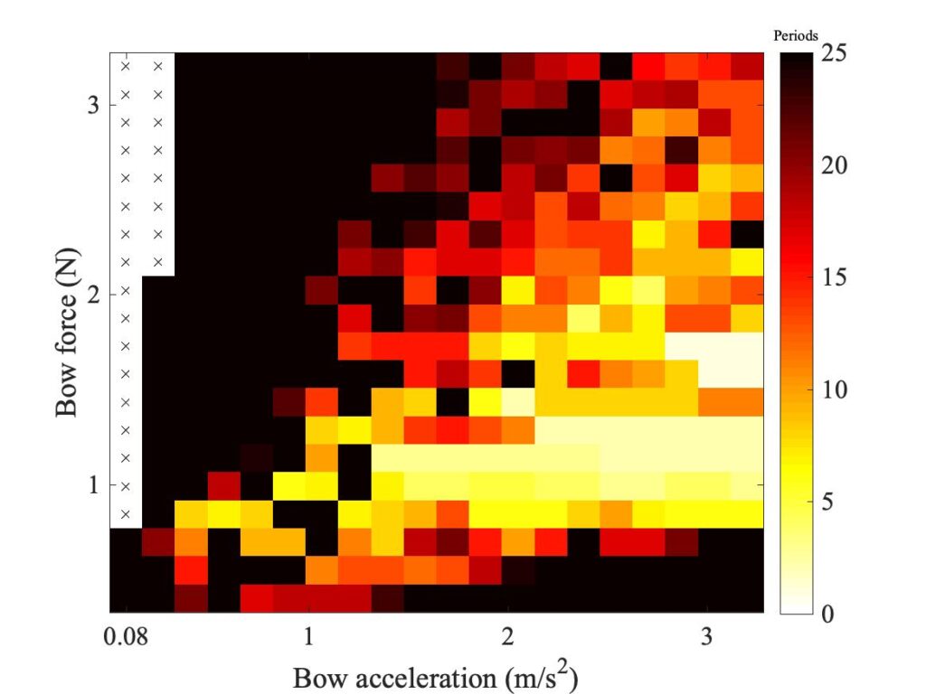
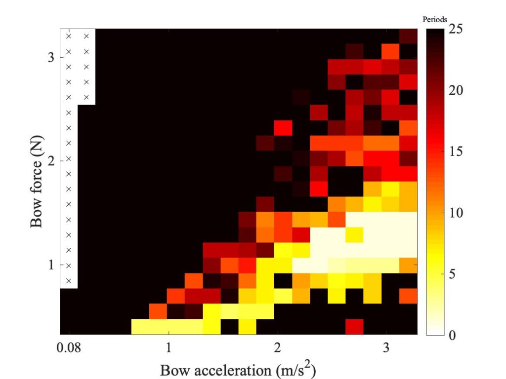
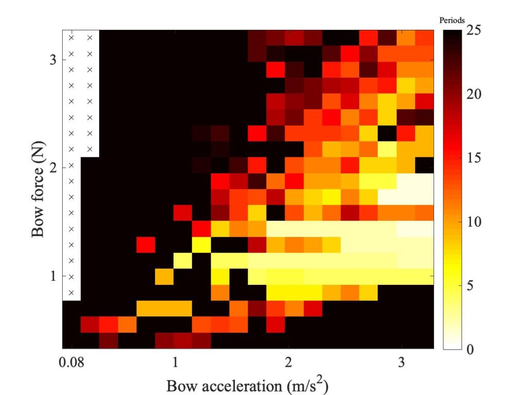
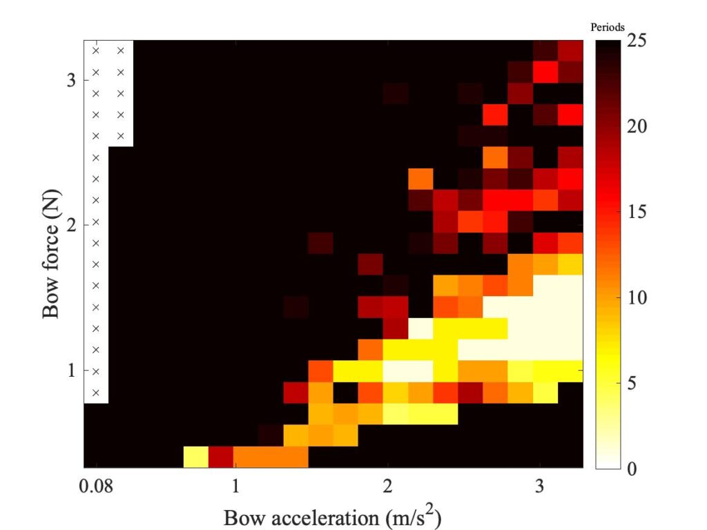
Figure 18 shows the effect of changing the thickness of the rosin layer in the model. The datum case used a thickness 1 $\mu$m, and this plot shows the effect of doubling (top row) or halving (bottom row) that thickness. The differences are very slight — it appears that the value of this parameter does not make very much difference, at least as assessed via the Guettler diagram.
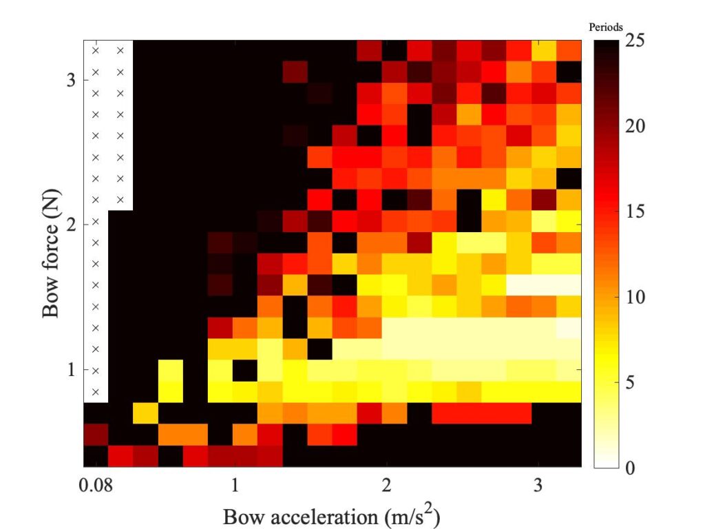
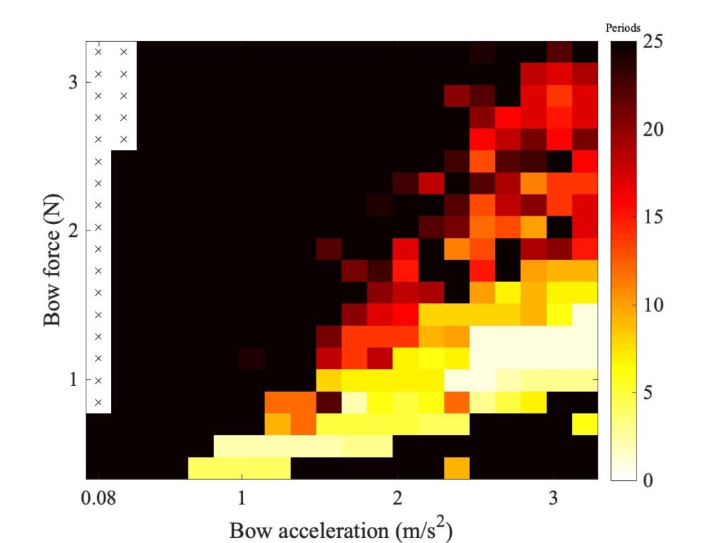
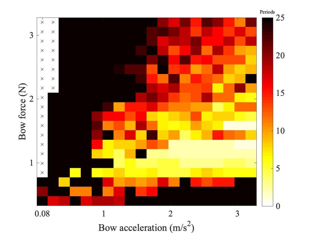
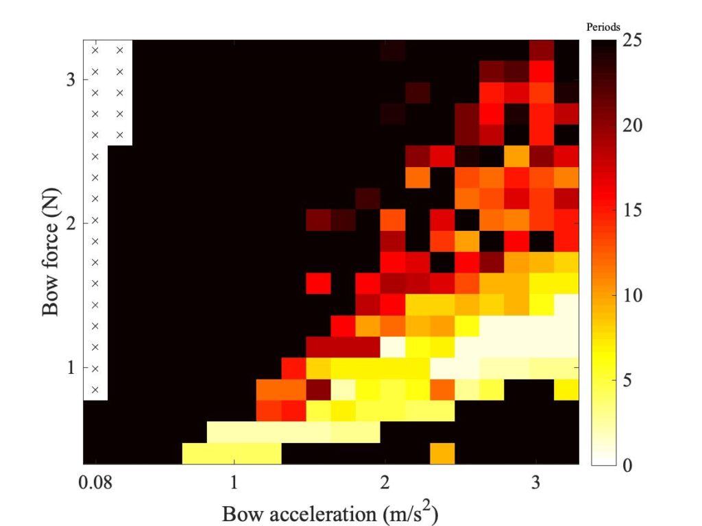
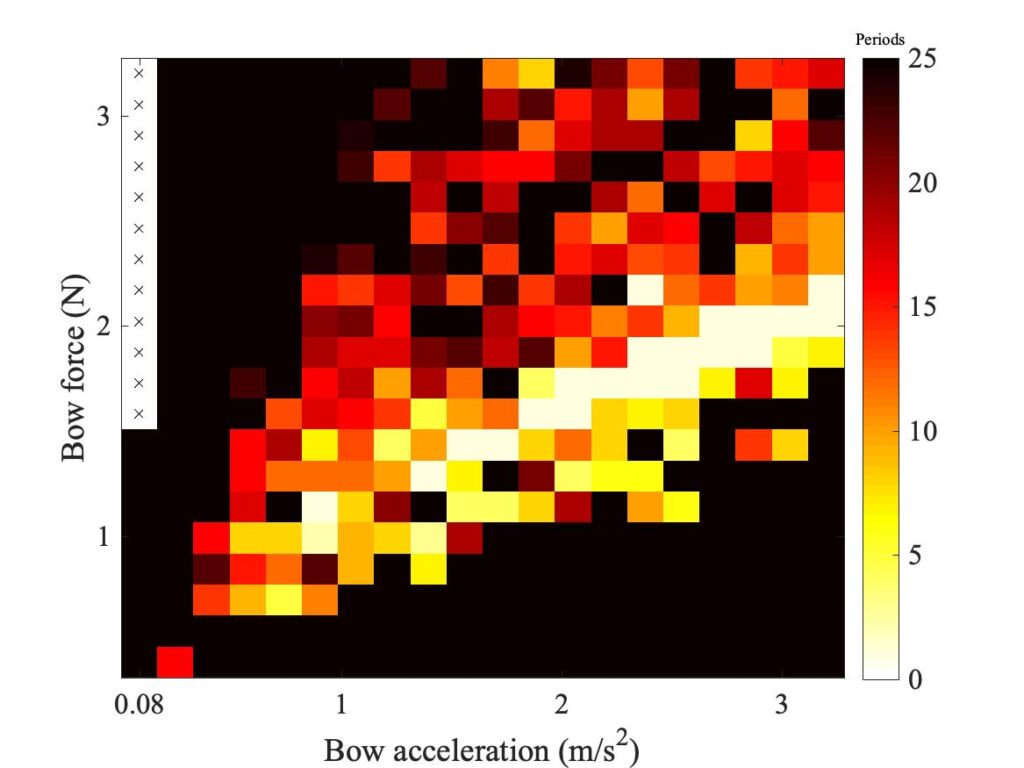
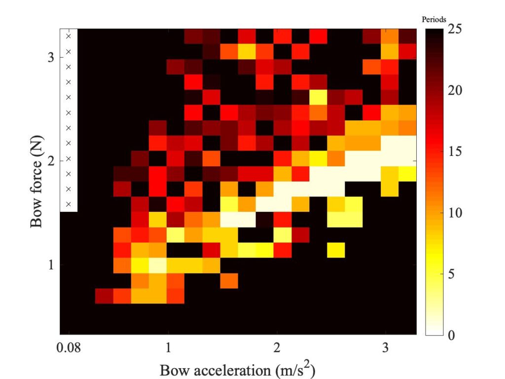
Figure 19 shows the influence of a different kind of variation of the frictional behaviour. All the results so far have assumed Coulomb’s law: the frictional force has been proportional to the bow force. But in section 9.6 it was pointed out that for the experiments with rosin-coated rod, and to lesser extent with the real bow, we might expect behaviour closer to “Hertzian contact” in which friction force varies with the 2/3 power of the bow force, rather than being directly proportional to it. As was anticipated in Fig. 3 of section 9.6, the edges of the region of coloured pixels tend to become upwardly curved rather than straight.
The next three variations to be explored involve a different aspect of the model: not the frictional behaviour, but the vibration response of the string and cello body. The model is based on the properties of a particular type of cello string, and the measured bridge admittance of a particular cello body. The body measurement, and a modal fit to that measurement, was carried out by Hossein Mansour. This was not the same cello that was used in the Galluzzo experiments, so we need to check whether that matters very much. Figure 20 shows a comparison of the two bridge admittances, and it also marks the first few overtone frequencies of the string used in the bowing experiments. The two cellos are obviously different, but the general level and shape of the two admittances is very similar.
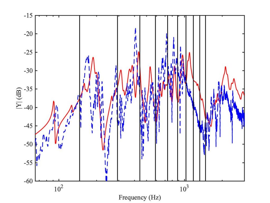
Figure 21 shows the results for the Guettler diagram when the cello body is assumed to be rigid (i.e. when the bridge admittance is set to zero). This is a far more drastic change than substituting one bridge admittance for the other from Fig. 20. It makes rather little difference to the result for the original thermal model, but for the enhanced model the region of coloured pixels is somewhat reduced.
Coupling the string to the cello body will have two effects: it will add damping, and perturb the overtone frequencies slightly. One would guess that the damping effect is the more important (noting that the chosen note on the cello is deliberately not near a strong resonance that might create a wolf note). Figure 22 shows the Q-factors of the first few string overtones with the body coupling (red squares), and with the rigid bridge assumption (blue squares). This confirms that the body coupling makes a very significant difference to the string damping, especially at lower frequencies.
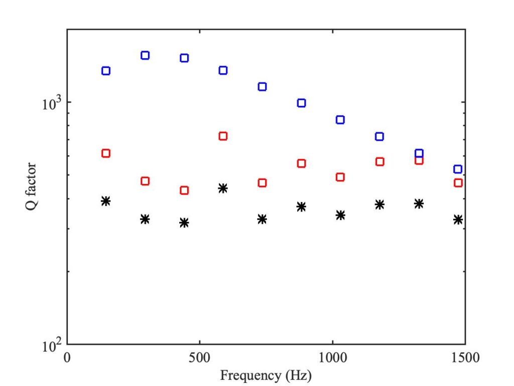
This plot also shows the effect of the next variation to be tested. The black stars show how the Q-factors change when the string is assumed to be finger-stopped, rather than an open string. This allowance for finger-stopping is based on the work of Suemae Saw [3]. Figure 23 shows the Guettler diagrams for this finger-stopped case. The comparison with Figs. 21 and 15 suggests that additional string damping tends to improve playability. Of the three cases, the finger-stopped string shows the largest regions of coloured pixels, the datum case is in the middle, and the rigid case from Fig. 21 shows the smallest regions.
The final case to be illustrated also involves string damping, in a rather indirect way. Figure 23 shows the Guettler diagrams for the case in which torsional motion of the string is suppressed. Torsional modes of the string have higher damping than transverse modes, so one effect of coupling is to add another source of energy dissipation. The interaction between transverse and torsional waves in the string is complicated, though, so it would be hard to guess the net effect. Indeed, the impression from this figure is that the effect on the two models is different. The Guettler diagram for the original thermal model, on the left, looks rather smoother and less speckly than for the datum case. But the right-hand plot for the enhanced model shows more black pixels in the middle of the region which is otherwise “playable”.
There is another issue concerning torsion that will become relevant in section 9.7, when we look into the effects of the finite width of the bow. For housekeeping reasons to do with the computer simulation code, it will be convenient to alter the torsional wave speed, so that the time delay for a torsional wave travelling across the bow is a bit longer. It is useful to give a direct comparison of the two speeds here, while we are talking about parametric variations. The discussion in section 9.7 will concentrate on the same value of $\beta$ as was used in section 9.6: it is the value from Fig. 5. Figure 24 shows a comparison of Guettler diagrams for the enhanced thermal model: on the left is a repeat of the bottom right-hand plot of Fig. 5, while on the right is the same case with the reduced value of torsional wave speed. The general region containing coloured pixels is similar in the two cases, but there is an obvious shift in the position of the white region.
Finally, another issue that will be relevant in section 9.7 concerns the sampling rate used in the simulations. All the results shown so far have used the rate 60 kHz, but for simulating a bow of finite width a higher sampling rate will be desirable. Figure 25 shows a comparison of Guettler diagrams generated with three different values of this sampling rate. The general shape is the same in all three plots, but the details change and the degree of “speckliness” increases. These plots illustrate “sensitive dependence” in action.

C. Parameter values and a few details
It is useful to summarise some details of the thermal models, in order to provide a full list of parameter values and also to highlight the known shortcomings of the current models so that we are not tempted to over-interpret or to expect too much of them. Both models assume that the interaction with the bow can be regarded as occurring at a single point on the string. The string’s vibration behaviour is then entirely captured by a single-point linear theory that links the surface velocity to the friction force. In the simulation, that theory is implemented via the “digital waveguide” methodology. Incoming transverse and torsional waves from the two sides of the bow are calculated from the corresponding outgoing waves by a process of convolution.
In parallel with this mechanical simulation, a temperature simulation is also carried out. The method is exactly as described in [2], except for a small extension to allow a non-circular contact footprint. We assume an elliptical contact region, with semi-axes $a$ in the direction of sliding and $b$ in the perpendicular direction (parallel to the string). The contact area is thus $A=\pi a b$. If the thickness of the rosin layer is $\delta$, the volume of rosin in the contact zone is $A \delta$. We can carry out a simple heat balance to calculate the average temperature of this volume.
Heat is generated by friction during sliding, at a rate
$$Q=F v \tag{1}$$
where $F$ is the friction force and $v$ the relative sliding speed. There are three effects balancing this heat gain. Conduction into the surrounding surfaces is modelled by the one-dimensional diffusion equation, on the assumption that the thickness is small compared to $a$ and $b$. The rate of heat loss by this mechanism, $Q_{cond}$, is proportional to $A$, and its calculation involves a Green’s function described in detail in [2]. Convolution with that Green’s function is carried out for the average time a particle of rosin spends within the contact patch: this transit time is
$$\dfrac{8a}{3 \pi v} . \tag{2}$$
Heat is also lost by advection, as warmed rosin is carried out of the contact region while cold rosin is carried in on the other side of the contact patch. The projected area through which this heat flow occurs is $2 b \delta$, and if the rosin layer is shearing uniformly through its thickness, the average transport speed is $v/2$. It follows that the rate of heat transport is
$$Q_{adv} = v b \delta \rho_r c_r T \tag{3}$$
where $\rho_r$ is the density of rosin, $c_r$ is its specific heat capacity and $T$ is the temperature above ambient that we are trying to calculate.
Finally some heat is absorbed by heating of the rosin within the contact volume, at rate
$$Q_{abs} = A \delta \rho_r c_r \dfrac{dT}{dt}. \tag{4}$$
The governing equation for $T$ then follows from the requirement
$$Q= Q_{cond} + Q_{adv} + Q_{abs} . \tag{5}$$
If the bow force $F_b$ changes, we scale $a$ and $b$ appropriately: for Coulomb’s law we need
$$a, b \propto F_b^{1/2} \tag{6a}$$
while for Hertzian contact we need
$$a, b \propto F_b^{1/3} . \tag{6b}$$
The simulations for the original thermal model are initialised at ambient temperature, but the simulations for the enhanced model are held at the crossing temperature $T_0$ (see section 9.6.2) until the first slip occurs. This is a blatant fudge, not claimed to represent the true physics, but it is necessary to make this model work as planned as a representation of the observed bridge force jumps.
For reference it is useful to list the parameter values used in the simulations, for the datum case. The contact parameters ($a$, $b$ and $\delta$) are needed for the bowed string and also for the steady-sliding experiment. (The steady sliding results are used in the calculation of the relationship between sliding speed, yield stress and temperature.) Table 1 gives all the values relevant to the frictional contact.
| Contact dimension $a$ for 1 N normal force | 0.26 mm |
| Contact dimension $b$ for 1 N normal force | 0.26 mm |
| Rosin layer thickness $\delta$ | 1 $\mu$m |
| Rosin density $\rho_r$ | 1010 kg/m$^3$ |
| Specific heat capacity $c_r$ | 250 J/kg/K |
| For the steady-sliding experiment: | |
| Contact dimension $a$ | 0.5 mm |
| Contact dimension $b$ | 0.5 mm |
| Rosin layer thickness $\delta$ | 2 $\mu$m |
| Normal force | 3 N |
Table 2 gives the parameter values for the cello string used in the bowing experiments. The damping of the string, apart from the contribution arising from coupling to the cello body, is described using a model due to Valette [4]: the Q-factor of the $n$th string mode with rigid terminations is
$$Q_n = \dfrac{P+EI(n \pi/L)^2}{P( \eta_F +\eta_A / \omega_n) + EI \eta_B(n \pi/L)^2}$$
where $P$ is the string tension, $L$ is its length, $EI$ is its bending stiffness, $\omega_n$ is the radian frequency of the mode, and $\eta_F$, $\eta_A$ and $\eta_B$ are three constants. For the calculation involving a finger-stopped string (Fig. 23), the constant $\eta_F$ was multiplied by a factor 3, as suggested by Saw [3].
| Fundamental frequency | 146.8 Hz |
| Tension $P$ | 111 N |
| Mass per unit length | 2.7 g/m |
| Transverse impedance | 0.55 Ns/m |
| Bending stiffness $EI$ | 3$\times$10$^{-4}$ N/m$^2$ |
| Damping constant $\eta_F$ | 2.3$\times$ 10$^{-4}$ |
| Damping constant $\eta_A$ | 0.11 s$^{-1}$ |
| Damping constant $\eta_B$ | 0.125 |
| Torsional to transverse wave speed ratio | 5.2 |
| Torsional impedance | 1.8 Ns/m |
[1] Knut Guettler, “On the creation of the Helmholtz motion in bowed strings”; Acta Acustica united with Acustica, 88, 970–985 (2002).
[2] J. H. Smith and J. Woodhouse, “The tribology of rosin”; Journal of the Mechanics and Physics of Solids, 48, 1633–1681 (2000).
[3] Suemae Saw; “Influence of finger forces on string vibration”, MEng dissertation, Department of Engineering, University of Cambridge (2010).
[4] C. Valette and C. Cuesta, “Mécanique de la corde vibrante”, Hermés, Paris (1993). A summary in English is given in C. Valette, “The mechanics of vibrating strings”, Chapter 4 of “Mechanics of musical instruments”, ed. A. Hirschberg, J. Kergomard and G. Weinreich; CISM Courses and Lectures no. 355, Springer-Verlag (1995).