
A. Differential slipping and “spikes”
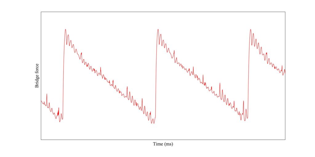
One thing missing from the simulation models used so far is the influence of the finite width of the ribbon of bow-hair — the models have all assumed a single point of contact between bow and string. The most obvious effect of finite width is best introduced by an example. Listen to Sound 1: this is a recording using a bridge-force sensor on the open G string of a violin. The player gradually slides the bow towards the bridge, getting very close at the end of the sample. In the sound, you should be able to hear a growth in harshness of the sound, ending with a definite “crunch”. This example is intentionally extreme, but players sometimes make deliberate use of this harsh sound at moderate level.
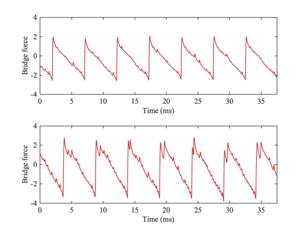
Figure 1 shows two extracts from this measured waveform, from early and late in the sequence. Both show the familiar Helmholtz sawtooth waveform, but they both have something extra superimposed. The upper trace shown occasional small spikes in the waveform, which differ in detailed placement from cycle to cycle. The lower trace shows a similar thing in more extreme form: it is not surprising that this irregular waveform might sound harsh or noisy.
We get a clue about what might be happening from Fig. 2. The upper diagram shows the moment in an ideal Helmholtz motion when the travelling corner has just gone past the bow, setting off towards the player’s finger. The ribbon of bow-hair is indicated by the yellow stripe: deliberately shown very wide, to make the effect clear. The lower diagram shows what might happen later in the cycle, shortly before the Helmholtz corner gets back to the bow. In the ideal version of Helmholtz motion, the string shape would follow the dotted line. But if the portion of string in contact with the bow has been sticking throughout this time, over the entire width of the bow-hair, the string would need to take up a zig-zag shape more like the solid line.
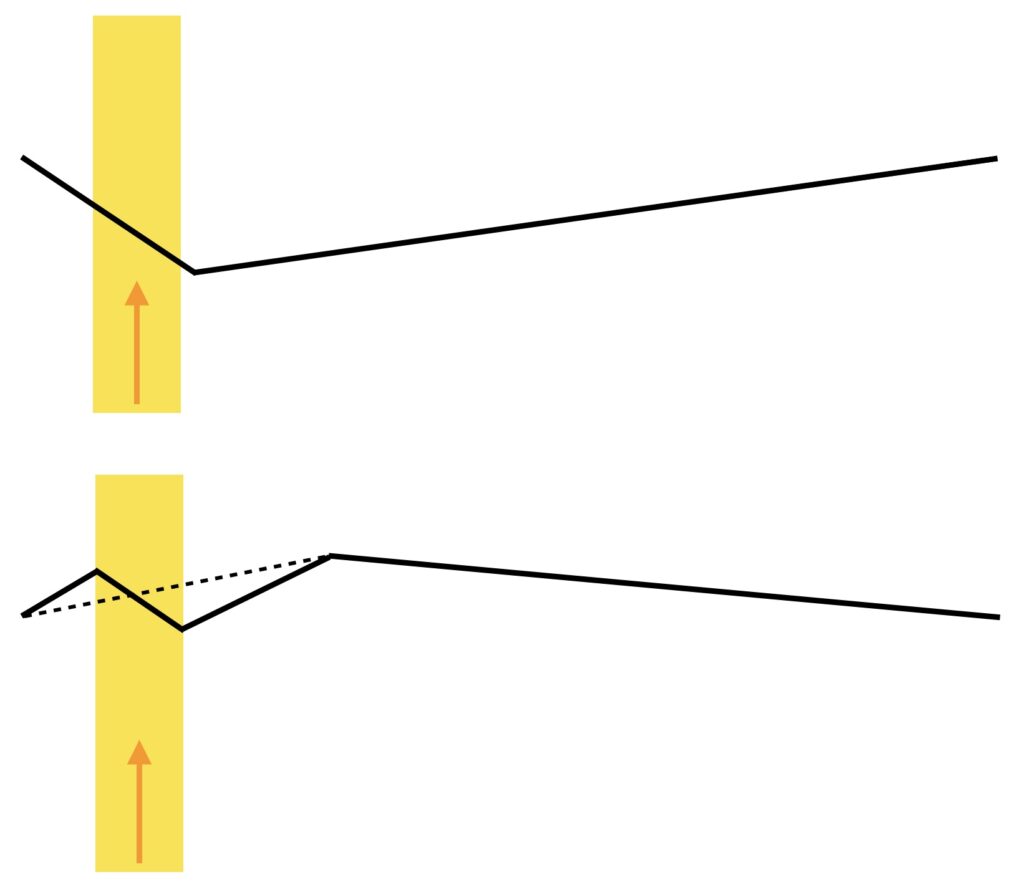
There are sharp corners at the edges of the bow-hair. These produce concentrated forces, in opposite directions on the two edges. This feels physically unrealistic: surely we might expect the string to have slipped in some region near the edges of the bow, before things got this extreme? Those localised slips, at the edge of the bow facing towards the bridge, are responsible for the “spikes” we saw in the bridge-force waveforms of Fig. 1. The effect becomes more extreme when the bow moves closer to the bridge.
We can confirm this idea by extending the computer simulation model to allow for a bow of finite width. Finite-width bowing has been most thoroughly investigated by Roland Pitteroff [1,2]. He included effects such as the elasticity of the bow-hairs, but unfortunately the approach he used cannot readily be combined with the simulation model we have used earlier (developed by Hossein Mansour [3]), for reasons of numerical stability. So instead, we use a simpler model which harks back to the earliest work on this topic [4], around 1980. It assumes a rigid bow, but one which contacts the string at several points rather than a single point. This model will allow us to make direct comparisons with the earlier simulations and the Galluzzo measurements, both based on bowing a cello D string. Some details are given the next link: the model is a straightforward extension of the point-bow model used earlier, so we can make direct use of the same friction models introduced in section 9.6.
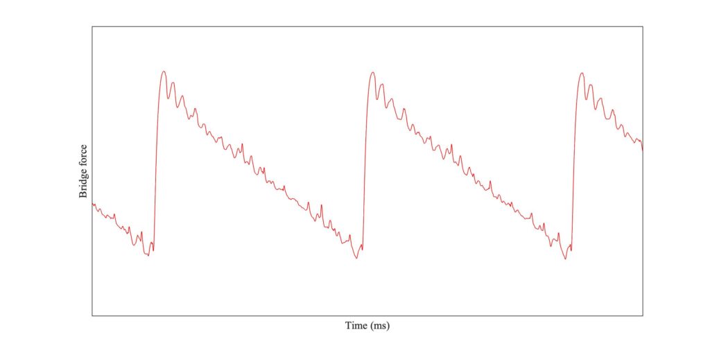
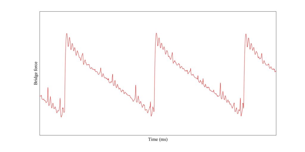
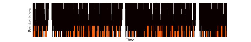
Figure 3 shows one example of such a simulation, using 6 “bow-hairs”. This particular example was made using the enhanced thermal friction model, initialised with ideal Helmholtz motion and then allowed to run for a while for the motion to settle down. The bridge force waveform shows an irregular pattern of spikes superimposed on a more-or-less steady Helmholtz sawtooth, qualitatively similar to the results in Fig. 1.
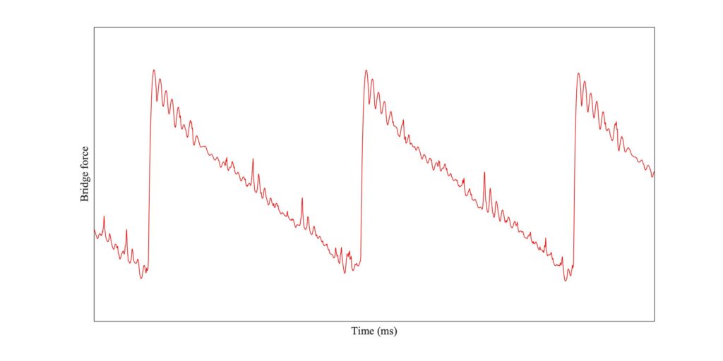
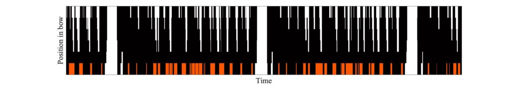
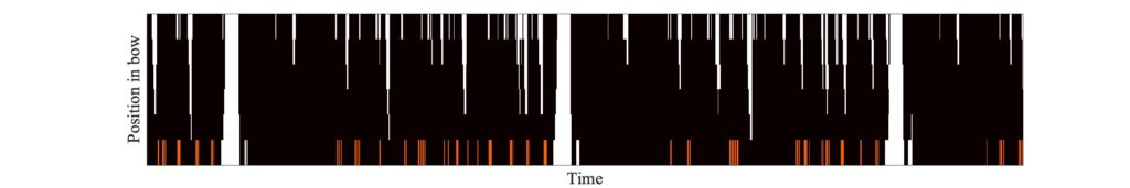
Figure 4 shows the corresponding pattern of sticking and slipping across the width of the bow. The time axis matches Fig. 3, and the top edge of the plot corresponds to the edge of the bow closest to the bridge. Black pixels indicate sticking and white ones indicate slipping. The main Helmholtz slips show up as top-to-bottom white stripes, while the partial slips causing the spikes in Fig. 3 show up as white streaks in the upper part of the plot. There are a small number of red pixels, indicating slipping in the reverse direction: these occur occasionally near the bottom edge of the plot, as Fig. 2 might have led us to expect.

B. The effect on Schelleng’s diagram
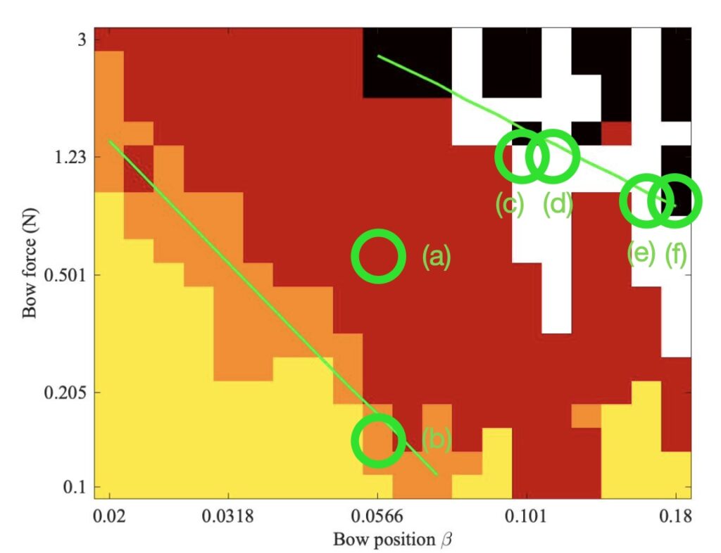
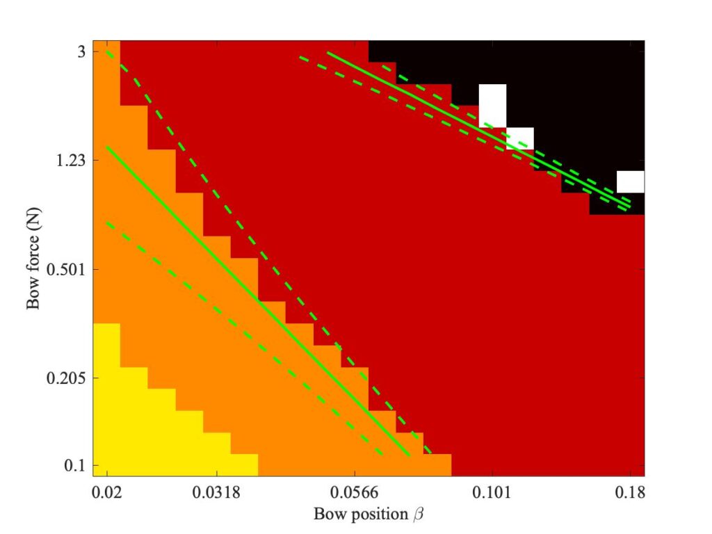
The same computational approach can be used to explore the effect of finite bow width on the behaviour in the Schelleng diagram. Simulations initialised with ideal Helmholtz motion can be made at a grid of points in the Schelleng plane, with different values of bow force and bow position distributed on logarithmic scales to match the Galluzzo measurement. The result of that measurement was discussed back in section 9.3, and the main plot is reproduced here as Fig. 5 (with the addition of some mark-up in green, to be explained shortly).
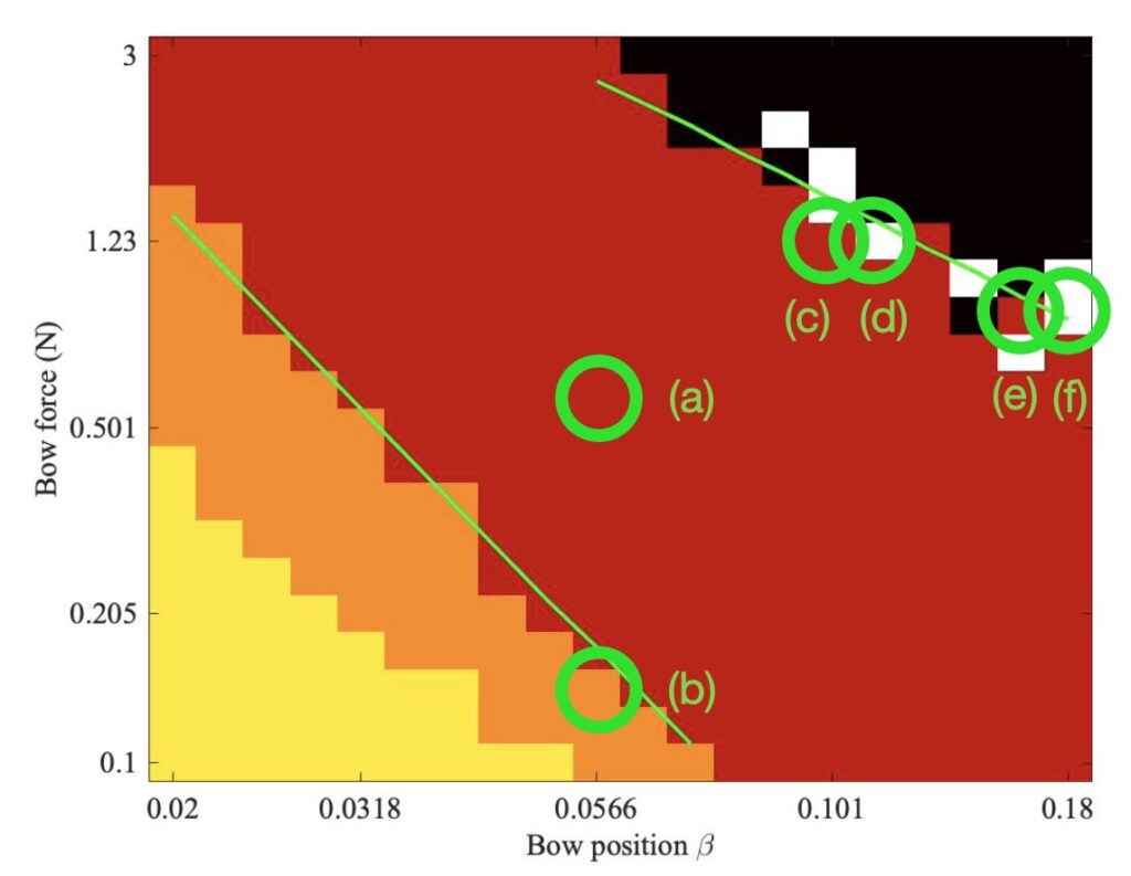
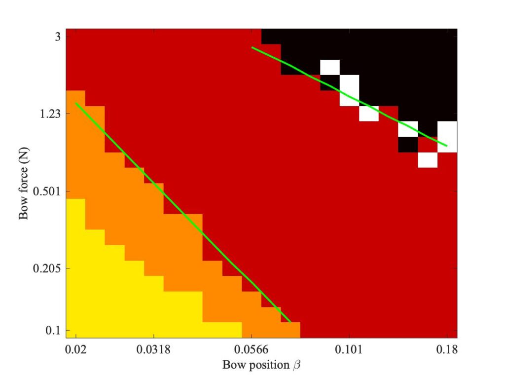
The measurements were made with the rosin-coated rod — unlike the Guettler measurements, they were not repeated using a normal cello bow. This means that direct comparisons with simulations will need to be with a point-bow model, but we can then use the finite-width simulations to indicate how things might change with a real bow. Figure 6 shows a Schelleng diagram simulated using a single-point bow and the enhanced thermal model of friction. Figure 7 shows the corresponding plot using 6 “bow-hairs” spaced over the 10 mm width of a cello bow, centred in each case on a nominal position indexed by the value of $\beta$.
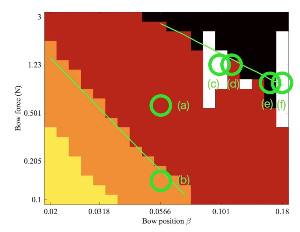
It is probably useful to start with a reminder of what we expect the Schelleng diagram to show, and what the different colours signify in these plots. All three plots show a central region of red pixels, connoting Helmholtz motion. Below the red pixels is a band of orange colour, connoting “double-slipping motion”, often described by players as “surface sound”. Below these orange pixels are some yellow ones, indicating a region where long-lasting steady stick-slip motion seems not to be possible at all — the string motion simply dies away.
On the opposite side of the region of red pixels, in the top right corner of all three plots, some black pixels can be seen. These connote non-periodic motion, described by Schelleng as “raucous”. Finally, there are some white pixels. These connote approximately periodic motion that is neither Helmholtz motion nor double slipping. We will see some examples shortly — they are all what Raman described as “higher types” of string motion, and are something players usually try to avoid unless they are deliberately seeking an unusual tone colour.
Schelleng predicted that the upper limit of Helmholtz motion, the maximum bow force, should follow a straight line in these log-log plots, with a slope of $-1$. The lower limit, the minimum bow force, should also follow a straight line, but with a steeper slope with the value $-2$. The two green lines marked in all three plots show what these slopes look like. The specific lines were fitted to the simulated results in Fig. 6, then the same lines are included in the other two plots.
We can learn some interesting things from these lines. First, it is by no means obvious that Schelleng’s argument will really apply to our thermal friction model, and even less obvious that it will apply to the finite-width simulations. But in fact Figs. 6 and 7 both show the red-orange boundary tracking the lower green line quite closely, and the red-black boundary tracking the upper green line moderately well. It looks as if the pattern of Schelleng’s limits continues to apply, and that a finite-width bow makes rather little difference to this aspect of behaviour. The regions of white pixels cut across the upper green line in Figs. 5 and 6, but that is to be expected. Versions of Schelleng’s calculation can be constructed for the various “higher types”, and this is the predicted behaviour: each variety of “higher type” has its own maximum and minimum bow force, different from those for Helmholtz motion.
Comparing Fig. 5 with Fig. 6, we can see some strong similarities but also some differences. The red-orange boundary follows a similar trend to the green line, but it is displaced upwards a little. The precise shape of the red-black boundary cannot be seen very clearly, but it seems to be in a very similar position to the green line deduced from the simulations. Looking back to section 7.3.1 where Schelleng’s limits were derived, this pattern makes good sense. The maximum bow force only depends on the bow speed and position, and the properties of friction. Those quantities are all supposed to be well matched by the simulation. However, the minimum bow force also depends on an additional property, related to the damping of the string vibration. It would not be at all surprising if the simulations do not quite match the damping of the experimental string and cello. One component of that damping relates to energy loss into the cello body at the bridge, and the simulations are based on measurements of a different cello body (see Fig. 20 of section 9.6.3 for details).
One obvious difference between Figs. 5, 6 and 7 is in the number and positions of the white pixels. Figures 5 and 6 show a generic similarity, although the details do not exactly match. Both show two vertical columns of white, at high values of $\beta$. Figure 7 shows far fewer white pixels, and they do not form obvious columns in the same way. To see what lies behind these differences, we need to look at some waveforms in detail. Six pixels have been chosen, marked (a)—(f) in all three plots. Matching extracts of bridge-force waveforms for these cases are plotted in Fig. 8—10. In each plot, the waveforms are in the same order as Figs. 5—7: the measurement at the top, the single-point simulation in the middle, and the finite-width simulation at the bottom.
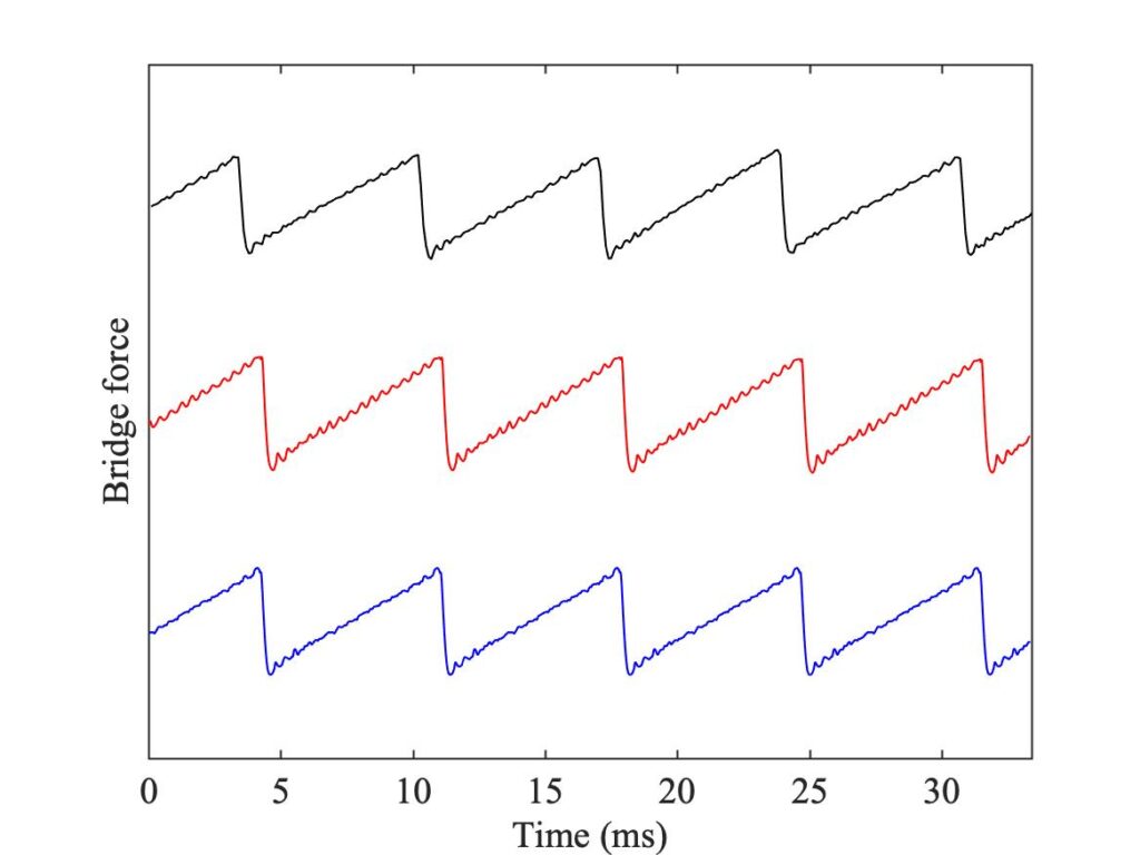
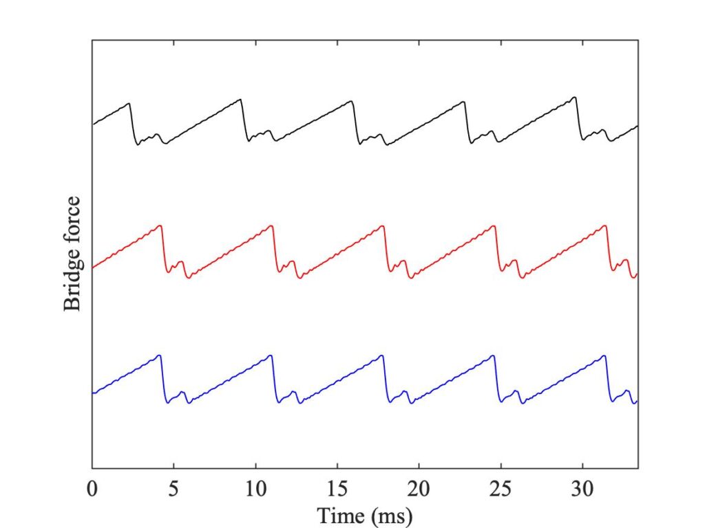
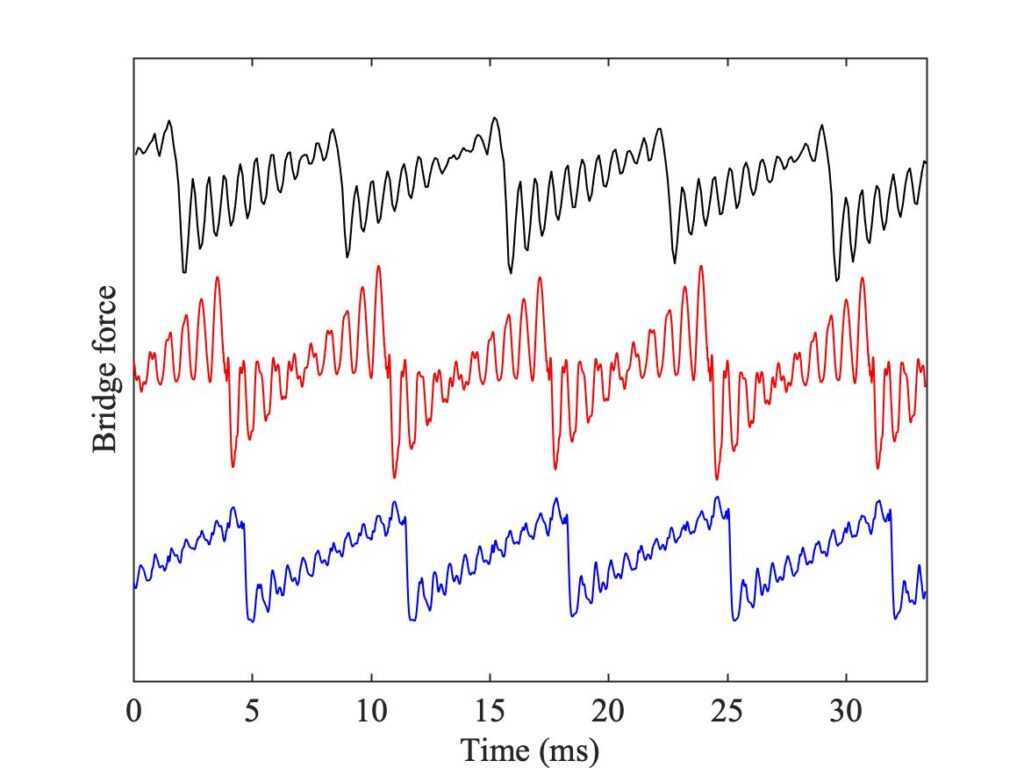
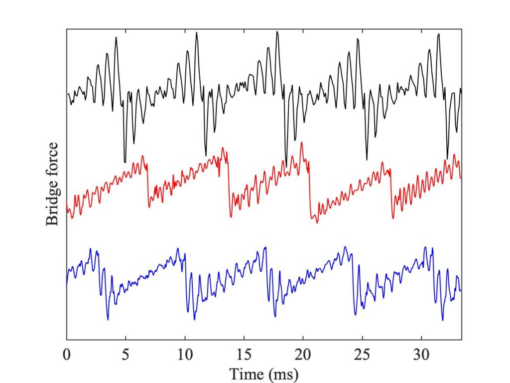
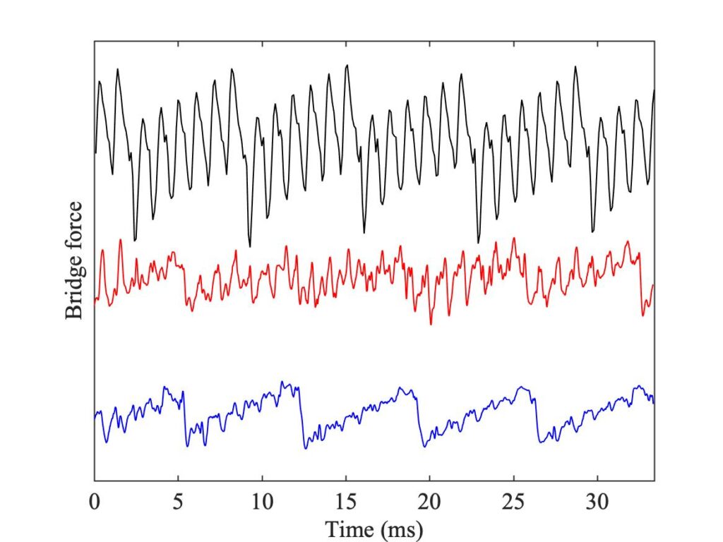
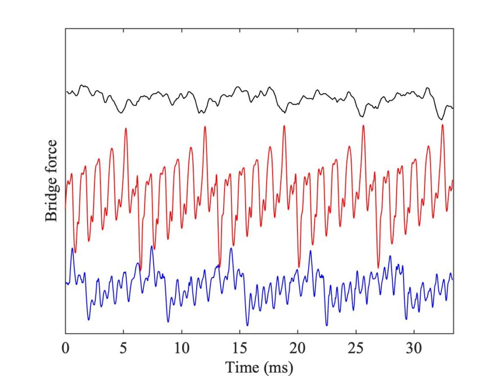
Figure 8 shows cases (a) and (b). Both points have been chosen to fall in regions with the same colour in all three Schelleng diagram. As expected, the left-hand panel shows Helmholtz motion, the right-hand panel shows double-slipping motion. For both of these, all three waveforms agree rather closely.
Figure 9 shows cases (c) and (d), placed in a region where white pixels appear. On the left, the measured waveform shows a “higher type” while the point-bow simulation shows a different one. The finite-width simulation shows Helmholtz motion, with a fairly well-developed pattern of Schelleng ripples. On the right, this figure shows a higher type in the measurement which is very similar to the one seen in the red curve on the left. The middle plot shows slightly irregular Helmholtz motion, and the lower plot shows yet another higher type, this one a variety of “double flyback motion”. Figure 10, showing cases (e) and (f), explores a different region of white pixels: it reveals a different mixture of higher types, along with Helmholtz motion and non-periodic raucous motion. This time, the measured waveform in the left-hand panel shows well developed “S-motion”, as does the middle waveform in the right-hand panel.
The conclusion from these plots is that the measurement shows a pattern of white pixels that is qualitatively similar to the single-point simulations. The precise position of the vertical columns is different in the two cases, but Figs. 9 and 10 suggest that the same repertoire of higher types is seen in both cases. With such a rich array of possible string motions, it is perhaps not surprising that there are detailed differences between measurement and simulation in terms of which regime occurs where.
The finite-width simulation (Fig. 7) shows far fewer white pixels, and thus a Schelleng diagram which is more orderly and closer to Schelleng’s original prediction. Somehow, the finite width is having an effect that tends to suppress higher types, which all involve large oscillations at the same frequency as the Schelleng ripples. Probably, players would welcome this difference. They are less likely to stray into unwanted S-motion or other higher types. Perhaps this is one reason for the use of a conventional bow, although there are many other reasons, some of them to be explored in the subsequent discussion.
There is another interesting thing to be learned from these simulations of the Schelleng diagram. Back in section 9.2, we saw a discussion of the effect whereby hysteresis in the friction behaviour during a cycle of Helmholtz motion can lead to pitch flattening of the note, especially when the bow force is high. The argument presented there was firmly based on the friction-curve model and a single bowing point, so it is interesting to explore whether the flattening effect is still predicted by a simulation model using the thermal friction model, and with a bow of finite width.
All the cases leading to red pixels in Fig. 7 were analysed in an attempt to extract the frequency of the Helmholtz motion. This was done by looking for the zero-crossings of the “Helmholtz flyback” in the bridge force over the final few period-lengths of each simulation. For cases identified clearly by the automated procedure, the averaged time interval between those zero-crossings was used to calculate a frequency, which was normalised by the nominal frequency of the fundamental resonance frequency of the string, 146.83 Hz. The results, expressed as a flattening in cents, are plotted in Fig. 11. The “floor” at $-10$ cents marks non-Helmholtz points.
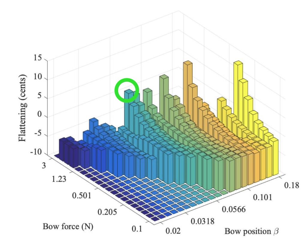
The results show a very interesting pattern. For values of $\beta$ above about 0.05, each line shows a steady rise as bow force increases. This is the “flattening effect” in action, more or less as the original argument suggested. But that argument does not predict the other obvious feature of the pattern: the plot reveals a remarkable sensitivity to the value of $\beta$, with the degree of flattening rising and falling in an apparently irregular way.
Notice that at the lower values of bow force, each line begins from a level with negative “flattening”. In other words, the note plays a little sharp relative to the frequency of the fundamental string resonance. This is probably caused by the influence of bending stiffness. Helmholtz motion always involves a significant contribution from higher overtones in the string motion, and in the free string those higher overtones are systematically sharp compared to a harmonic series based on the fundamental. The bowed string then chooses a “compromise pitch” that is slightly sharp, as these results show.
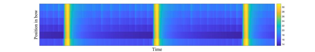
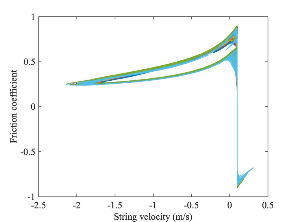
It is worth seeing some details for a typical example. The green circle in Fig. 11 marks a case showing significant flattening. Figure 12 shows the final bridge force waveform for this case, plus corresponding maps of the slip/stick state and the temperature distribution across the width of the bow. The temperature reaches a maximum of 31$^\circ$ above ambient, or 51$^\circ$C. Figure 13 shows a plot of the friction force (normalised by the normal force on each “hair”) against velocity. A separate line is plotted for each “hair”, but they all lie on approximately the same path. A hysteresis loop is seen, qualitatively similar to the one shown in Fig. 6 of section 7.6.
C. Tilting the bow
The finite-width bowing model allows us to make a preliminary exploration of something important. We have already discussed the effects of several variables a player can control during bowing: the bow force, speed and acceleration, and the position of the bow on the string. But there is another important variable, which we have ignored up to now: players do not necessarily press the bow-hair flat against string. Instead they usually tilt the bow, so that the distribution of normal force is not uniform across the width. The degree of tilt often varies in the course of each bow stroke, and in extreme cases it may be so large that the hairs only contact the string over a small part of the width. Manipulating bow tilt is a major ingredient of the player’s armoury, when striving to achieve subtleties of tone.
We will not attempt to model such subtleties here: instead, we will explore some of the simpler effects of bow tilt by comparing three idealised cases. The bow width in contact with the string will stay the same, but three different distributions of normal force will be used: uniform (the “flat bow”), or tapering linearly across the bow from near zero at one edge to a maximum at the other edge. This taper could go in either direction. Conventional tilt involves reducing the force on the side facing the bridge, and players do not ordinarily tilt in the opposite direction, so we will label these two cases “correct tilt” and “incorrect tilt”.
Figures 14, 15 and 16 give a first impression of the consequence of a tilted bow. Figure 14 repeats the plots from Figs. 3 and 4, with a flat bow. It shows Helmholtz motion, with some irregular “spikes” in evidence. Figure 15 shows the “correct tilt” case: all parameters are the same, except that the normal bow force varies linearly across the width of the bow, falling to zero at the edge nearest to the bridge and rising to double the mean level at the opposite edge. Figure 16 shows the converse case, with “incorrect” tilting so that the force is higher at the edge nearest to the bridge.

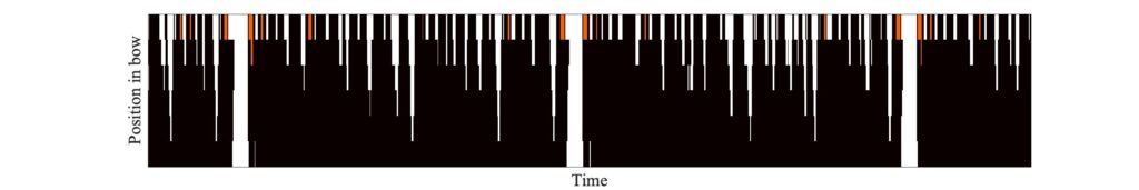
Comparing Figs. 14, 15 and 16, the bridge force waveforms look quite similar but the stick-slip patterns are significantly different. With the flat bow, the white streaks marking the partial slips responsible for the obvious spikes in the bridge force extend across almost the whole width of the bow. For the correctly tilted case the same is true, but now the edge of the bow nearest to the bridge is slipping for most of the time (occasionally in the reverse direction). For the incorrectly tilted case, the converse pattern is seen. The section of the bow facing the bridge is sticking most of the time, while the other edge is usually slipping, mostly in the reverse direction indicated by red points in the plot.
Figures 17, 18 and 19 explore the consequences of bow tilt for Schelleng’s diagram. Figure 17 shows a repeat of Fig. 7, for the flat bow; Fig. 18 shows the case with correct tilt; and Fig. 19 shows the case with incorrect tilt. The most conspicuous difference between these three plots is that the red-orange boundary and the red-black boundary have both shifted: downwards in Fig. 18 and upwards in Fig. 19. These shifts are due in part to a change in the “centre of gravity” of the normal force, from the centre of the bow-hair in the flat case towards one edge or the other in the tilted cases. To indicate the consequences of this shift, the green lines have been augmented by dashed lines indicating where they would appear for a single-point contact at the two extreme edges of the bow (but with the $\beta$ value on the horizontal axis still at the bow centre because the player hasn’t shifted the bow, they have only tilted it).
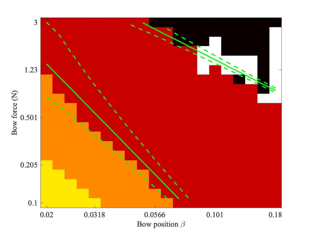
It is immediately clear that the shift in minimum bow force (red-orange boundary) is quite well captured by the dashed green lines. The boundary in the case with correct tilt approaches the lower dashed line, while in the case with incorrect tilt it approaches the upper line, very much as one would have guessed from the lower plots in Figs. 15 and 16. Correct tilt tends to increase the effective value of $\beta$, while incorrect tilt would tend to decrease it. The reduction in minimum bow force associated with correct tilting may point to one reason a player might use such tilting, if they want to play quietly.
The situation is somewhat less clear for the red-black boundary and the maximum bow force. Tilting in either direction makes relatively little difference to this limit, and the dashed green lines mark out a narrower band in the plot. However, there is another obvious difference between the Schelleng diagrams. Correct tilt leads to more white pixels, so using a tilted bow while playing far from the bridge makes it a little more likely that a higher type such as S-motion will be obtained, rather than Helmholtz motion. The conclusion is that a player wanting to use high bow force while maintaining Helmholtz motion probably needs to use a flat bow.
D. The effect on Guettler’s diagram
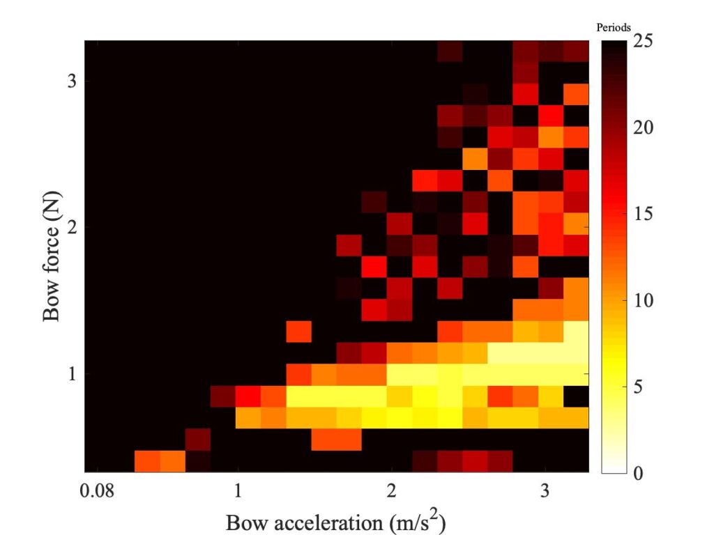
Having looked at the effects of finite width and tilt on the steady motion of a bowed string, we can now turn to transients and the Guettler diagram. Section 9.6.3 gave some detailed results comparing measurements with point-bow simulations, using the original and enhanced thermal models for friction. There are good reasons to expect the enhanced model to be closer to reality, but that section highlighted two areas where the original thermal model seemed to give better predictions than the enhanced model. The effects were shown most clearly at the largest value of $\beta$ from the measurements, so to see how these issues are impacted by finite bow width we will concentrate on this case with $\beta = 0.18$.
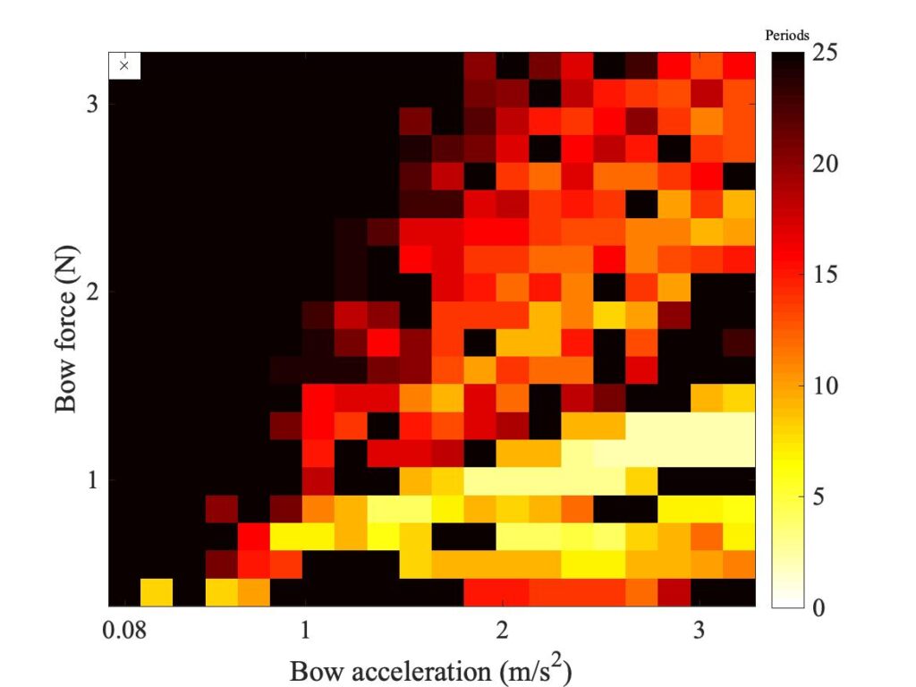
Figure 20 shows the relevant measurement, while Fig. 21 shows the corresponding simulated result using the point-bow model with the enhanced thermal friction model. Figure 22 shows a direct comparison using the finite-width model, with a flat bow. One of the two issues pointed out earlier is immediately obvious from the comparison of Figs. 20 and 21: there is far more “black space” in the upper left of Fig. 21. Figure 22 shows that the finite-width model has gone some way towards filling this in with coloured pixels. The colours in Fig. 22 are generally less bright than in Fig. 20, connoting somewhat longer transients, but the total area covered by coloured pixels is significantly closer to the measured case than was the case with Fig. 21.
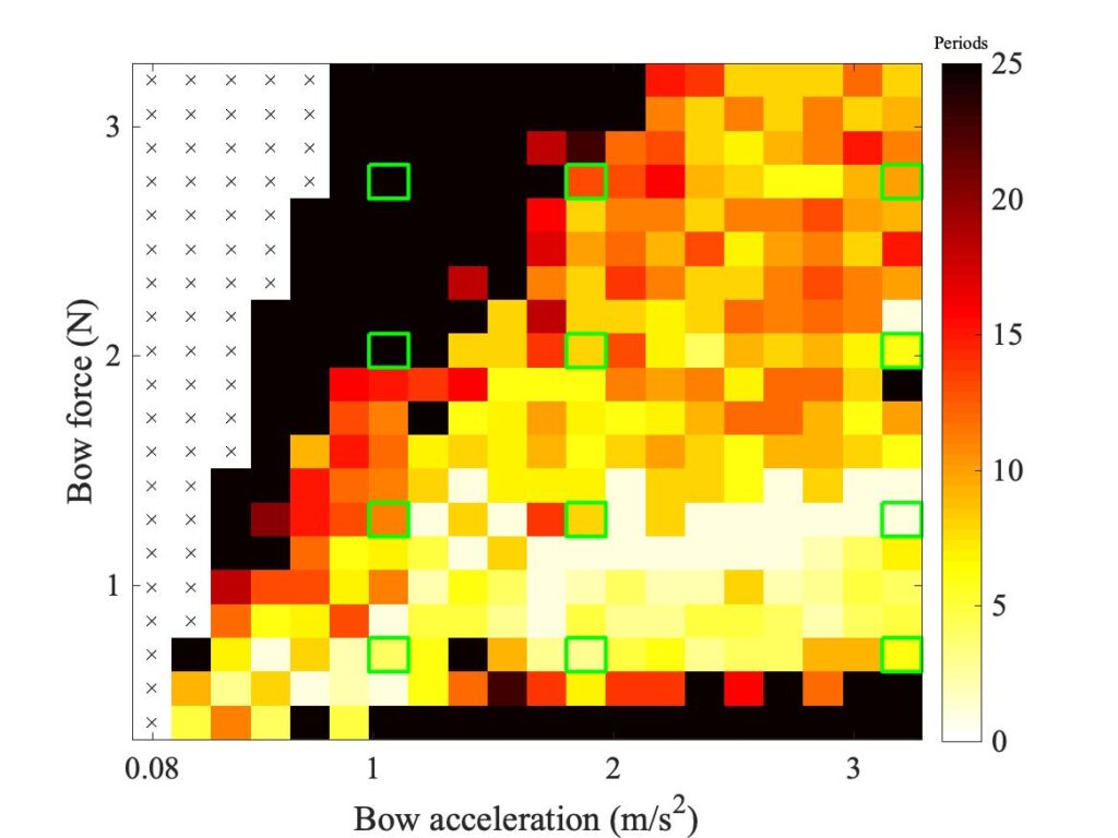
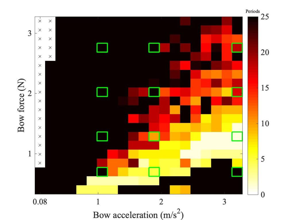
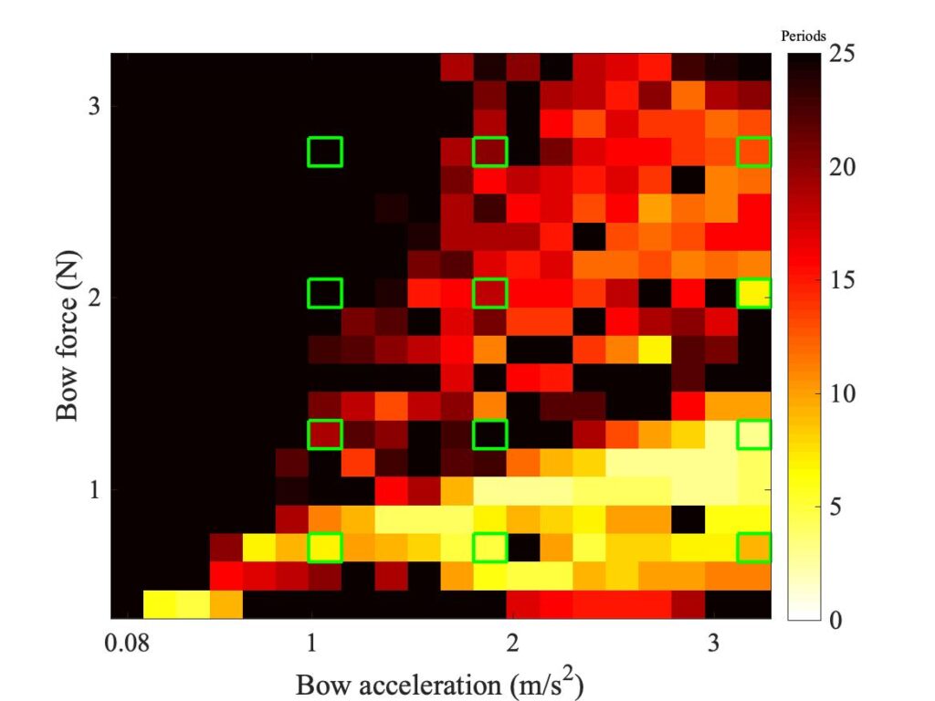
This is encouraging, but there is more good news when we dig into the waveforms lying behind these Guettler plots. Figures 20, 21 and 22 are all annotated with green squares, marking cases we will look at in detail. Figures 23, 24 and 25 then show comparisons of bridge-force waveforms for these cases, one column at a time. Specifically, they show a short extract towards the end of the measured interval, which was 0.25 s long. In each figure, the left-hand panel shows the comparison of the measurements (in black) with the simulations using the point-bow model (in red). The right-hand panel shows the corresponding comparison with the finite-width simulations. To aid comparison, all waveforms have been scaled to the same RMS value and the simulations have been phase-shifted if necessary to bring them into a best match with the measurement.
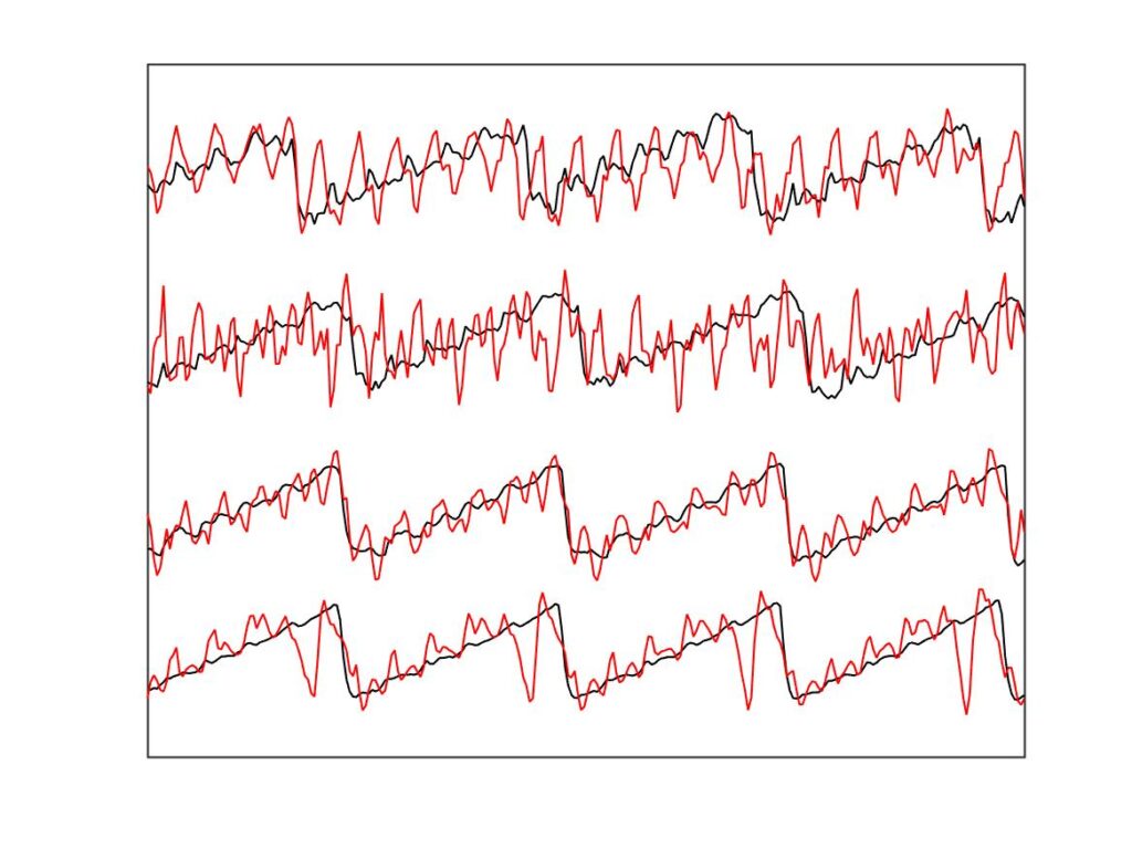
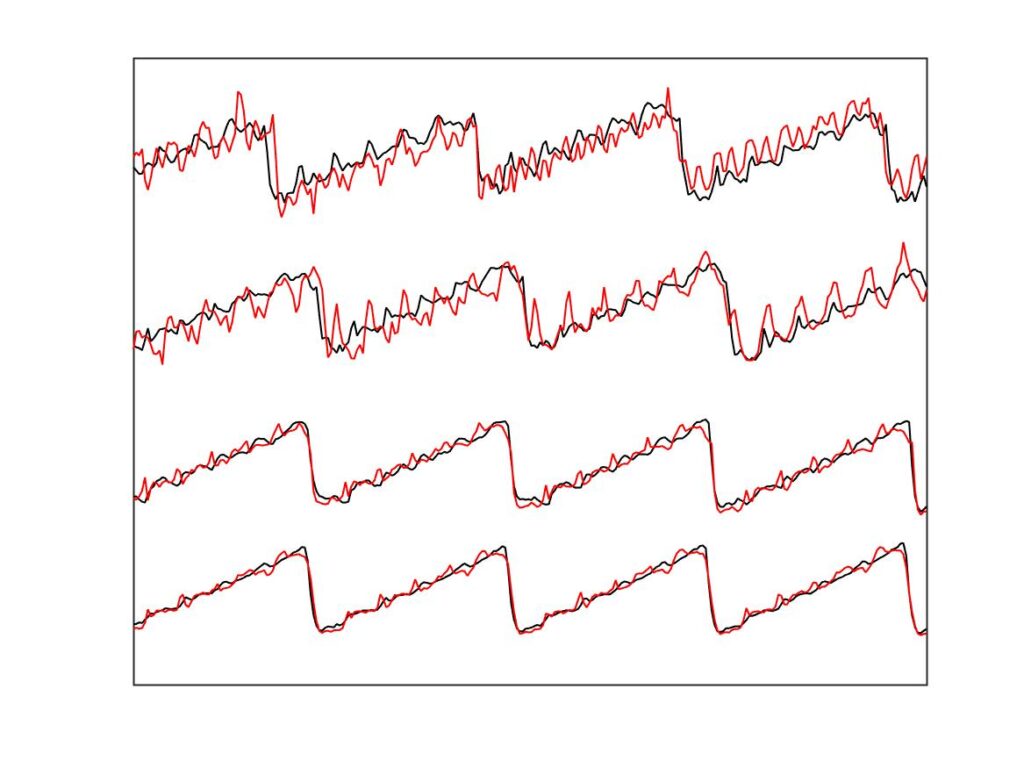
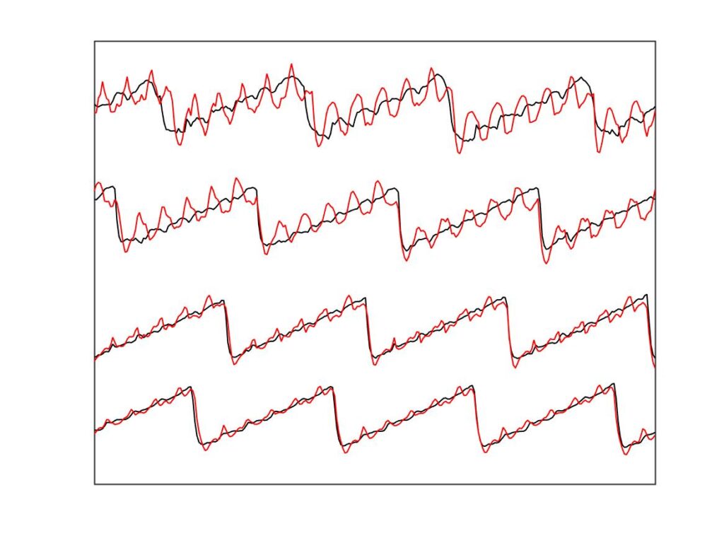
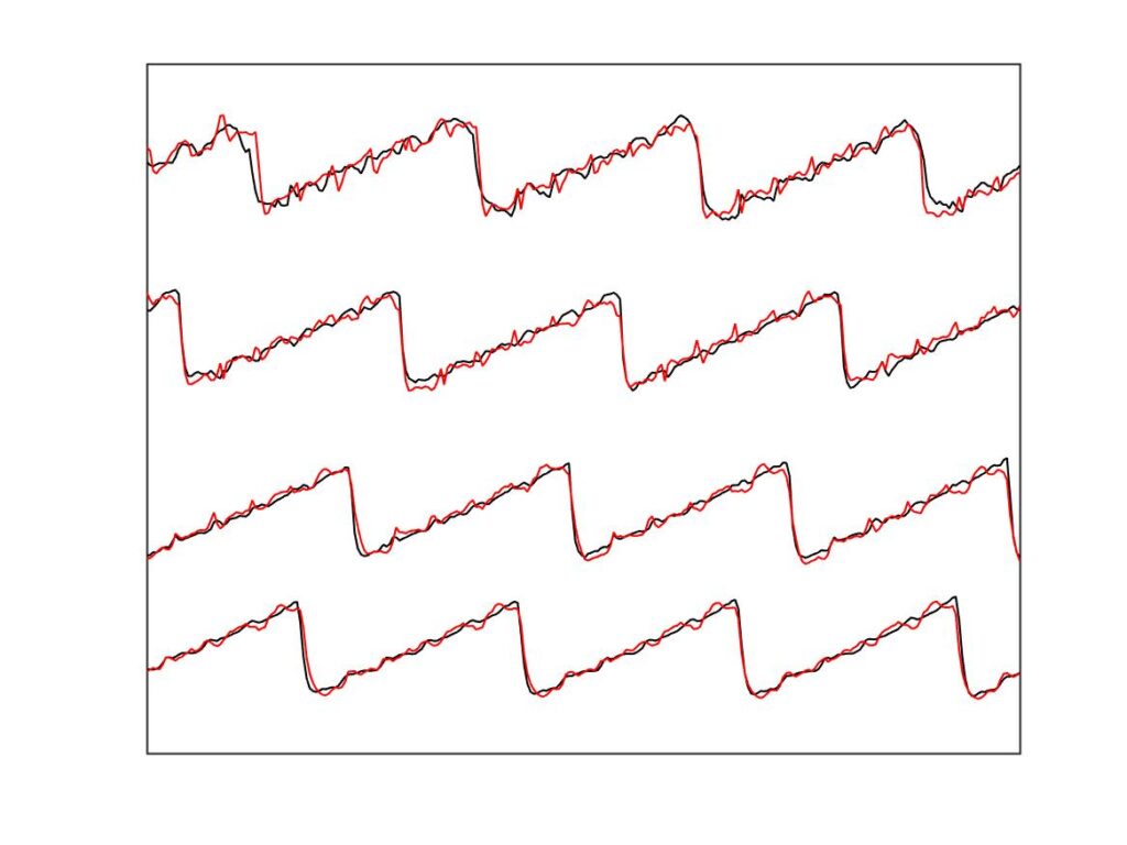
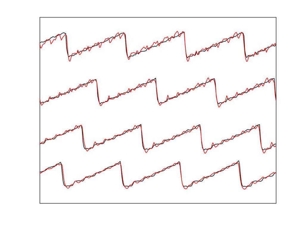
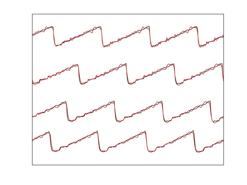
It is immediately clear that the finite-width simulations match the measurements much more closely than the point-bow simulations do. The contrast is most clear in Fig. 23, for the leftmost column of marked points in Figs. 20—22. For all four cases plotted, the point-bow simulation shows a “higher type” of one kind or another, whereas the measurement shows something close to the Helmholtz sawtooth. This is the second issue highlighted earlier: the enhanced thermal model seemed over-prone to higher types. With the finite-width simulations, on the right, the problem is substantially reduced: they show approximations to the sawtooth waveform in all four cases. The top two admittedly show a more marked pattern of “ripples” than the measurement, but nowhere near as prominent and disruptive as in the corresponding cases on the left.
The conclusion, backed up by inspecting a wider range of points in the Guettler diagram, echoes something found earlier in this section. Finite bow width tends to suppress oscillations which in extreme cases turn into undesirable higher types, and it does so in a way that seems to mirror the measurements fairly closely. In consequence, finite-width simulations based on the enhanced thermal model of friction seem able to give a reasonable match to all the available measurements. The match is by no means perfect, but it is by far the best so far achieved. More plots relating to Guettler transients with this model, including some comparisons between the original and enhanced thermal models, can be found in the previous side link.
We have commented already that Fig. 22 shows transient lengths that are usually a bit too long. A particularly striking example is given by the second waveform from the bottom in Fig. 24. The corresponding marker in Fig. 22 shows up as a black square, but Fig. 24 shows a Helmholtz sawtooth. The explanation is simply that this case did lead, eventually, to Helmholtz motion, but the transient was more than 25 periods long so it was not caught by the processing that generated Fig. 22. The same description is true of the other black or dark brown pixels that form an obvious stripe across Fig. 22. No such feature is visible in Fig. 20, so this is an example of something not well captured by the simulation model.
Finally, Fig. 26 shows what the simulation model predicts with a tilted bow. The left-hand Guettler plot shows correct tilt, the right-hand one shows incorrect tilt. Comparing these with Fig. 22, we can see that correct tilt generates a lot more black pixels in the upper left of the plot. Incorrect tilt has a less striking effect, and if anything it increases the area of coloured pixels a little. However, note that all three plots show the wedge of brightest pixels in a very similar position. This corresponds, more or less, to Guettler’s original analysis of “perfect starts”, and it looks as if bow tilt has rather little influence on that region of the player’s parameter space. But if a player wants to create Helmholtz motion efficiently with rather high force but low acceleration, they had better use a flat bow rather than a “correctly” tilted one.
[1] R. Pitteroff and J. Woodhouse, “Mechanics of the contact area between a violin bow and a string. Part II: simulating the bowed string”; Acta Acustica united with Acustica, 84, 744—757 (1998).
[2] R. Pitteroff and J. Woodhouse, “Mechanics of the contact area between a violin bow and a string. Part III: parameter dependence”; Acta Acustica united with Acustica, 84, 929—946 (1998).
[3] Hossein Mansour, Jim Woodhouse and Gary P. Scavone, “Enhanced wave-based modelling of musical strings, Part 2 Bowed strings”; Acta Acustica united with Acustica, 102, 1094–1107 (2016).
[4] M. E. McIntyre, R. T. Schumacher and J. Woodhouse, “Aperiodicity in bowed-string motion”, Acustica 49, 13—32 (1981). See also Erratum, Acustica 50, 294—295 (1982).