
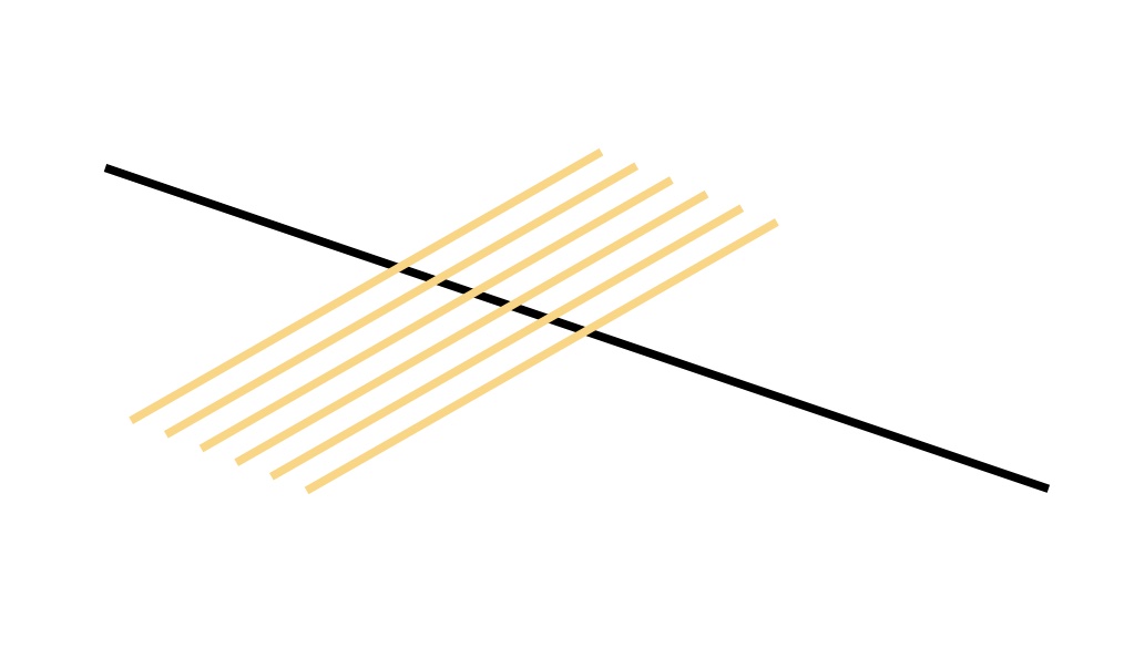
There are several possible ways to extend the bowed-string simulation model to allow for a finite-width bow. In the existing literature, the most thorough study was by Roland Pitteroff [1,2]. He assumed some number of separate, discrete “bow-hairs”, spread over a chosen total width as sketched in Fig. 1. These “hairs” were not assumed to be rigid: instead, measured behaviour of individual strands of horsehair was used to deduce an approximate model for each “hair” in the discrete model, consisting of a parallel spring-dashpot combination.
The model then used a finite-difference approach to the section of string lying under the bow, combined with the digital waveguide method to represent the two sections of string outside the width of the bow. At each time step, outgoing waves from the two edges of the bow were converted into incoming waves by convolution with reflection functions, exactly as in the point-bow model described earlier. The short section of string under the bow was treated in the simplest possible way: transverse and torsional waves were each assumed to obey the simple wave equation, with the appropriate wave speeds. Local effects of damping and bending stiffness within this short length were ignored: but for the string as a whole they were allowed for via the reflection functions.
Each wave equation was represented approximately by a central-difference form for the spatial second derivative, involving the displacements of the “hairs” on either side of the one being considered, and by a backward-difference form for the time derivative. The spring-dashpot model for the “hairs” was also expressed in a finite-difference form. Putting all this together, the new value of displacement of string and bow-hair at each discrete “hair” could be calculated, from a knowledge of the displacement of it and its neighbours at previous time steps together with the friction force acting on that particular “hair”. Details of all this can be found in reference [1].
For the present purpose, it is very desirable to use an approach that is based on the point-bow simulations we have seen earlier, so that we can get a direct impression of what changes when the bow width is made finite. Unfortunately, efforts to combine Pitteroff’s approach with the existing point-bow simulation ran into difficulties: one reason was associated with the digital filters used to represent the internal damping in the string, while another was associated with the fact that we want to apply the approach to a cello string in order to compare with the Galluzzo measurements.
Pitteroff’s work looked mainly at violin strings. An open cello string has a length around 680 mm, while an open violin string has a length around 330 mm. In normal bows the ribbon of hair is wider at the frog and narrower at the bow tip, but measured in the middle of the bow the hair width is about 10 mm for both a violin bow and a cello bow. This is a much bigger fraction of the string length for a violin than for a cello. Now, the resolution for the spatial variation within the bow width obviously depends on the number “bow-hairs” used. Having made that choice, there is a lower limit on the chosen sampling frequency (or equivalently, an upper limit on the time step length) in order to achieve numerical stability with the finite-difference method. It turned out that with cello-like parameter values, the required sampling rate became embarrassingly high, and the process of simulation became slow, unwieldy and inaccurate. Furthermore, Mansour’s algorithm for designing the digital filters for string damping [3] became unstable at this high sampling rate.
To resolve these difficulties, a simplified approach to simulation was developed. It still involves a number of discrete “hairs”, but these are now regarded as being rigid (as in the point-bow model from earlier sections). Instead of the finite-difference method, the digital waveguide approach was used to handle the dynamics of the string within the width of the bow. Each “bow-hair” generates outgoing transverse and torsional waves. Making the same assumption of simple wave propagation within the width of the bow, these waves reach the neighbouring “hairs” after a small time delay.
If that delay is longer than one time sample, a relevant incoming wave at an adjacent hair can be calculated, approximately, by linear interpolation based on earlier outgoing waves. Such interpolation proved to work well. However, there is a problem if the delay is shorter than one time sample. To apply the same approach we would need to extrapolate the earlier samples rather than interpolating them, and such extrapolation caused insuperable stability problems. For transverse waves, this issue was dealt with simply by choosing the sampling rate and the number of “hairs” so that it did not arise. The chosen sampling rate was 120 kHz, and with the parameters of the cello string this restricted the number of “hairs” to a maximum of 6 (the number illustrated in Fig. 1).
However, torsional waves have a higher propagation speed than transverse waves — 5.2 times higher for the cello string in the measurements. To cope with this, a more drastic approximation was needed. When the correct delay was less than one sample, the simulation avoided extrapolation by simply using a 1-sample delay. What this means in physical terms is that the torsional wave speed was made artificially slower within the 10 mm width of the bow. However, the torsional resonance frequencies were only affected very minimally, because the correct speed was used when calculating the reflection functions describing torsional wave propagation in the rest of the string — and recall that the bow occupies only 1/68 of the total length for an open cello string.
The calculation of the friction force at each “hair” involves nothing new: each is treated exactly like the single-point bow we have studied in earlier sections. Among other things, this means that we can use the same three friction models; the friction-curve model and the two thermal models. For the latter we perform separate temperature calculations for each “hair”, using the same method as in the point bow model.
We can illustrate some typical results of this model. The first step is to see what happens when a single-point model turns into ae finite-width model. Figure 2 shows a succession of simulated Guettler diagrams, all for bow position $\beta$ = 0.18 and computed using the enhanced thermal model. The top left panel is a repeat of the point bow result shown earlier. The remaining panels all show a “bow” of width 10 mm, with successively 2, 3, 4, 5 and 6 “hairs” distributed within that width. For 2 hairs, the torsional wave delay across the bow is more than one sample, so the “fudge” is not needed. But for all the other cases this is not the case.
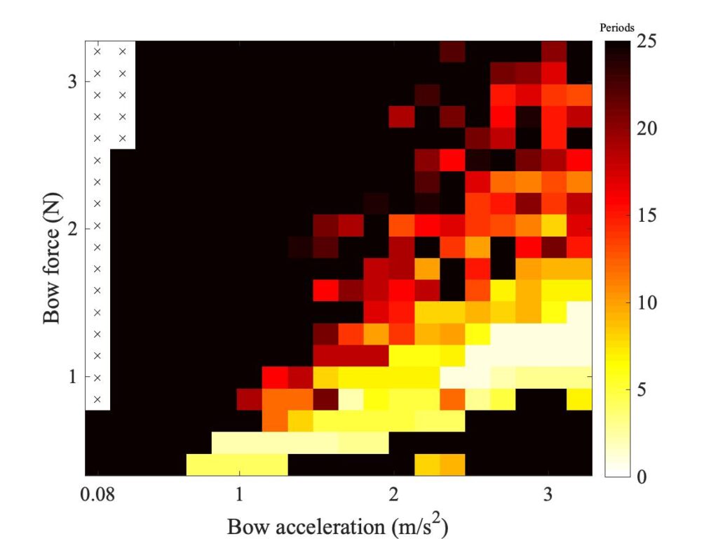
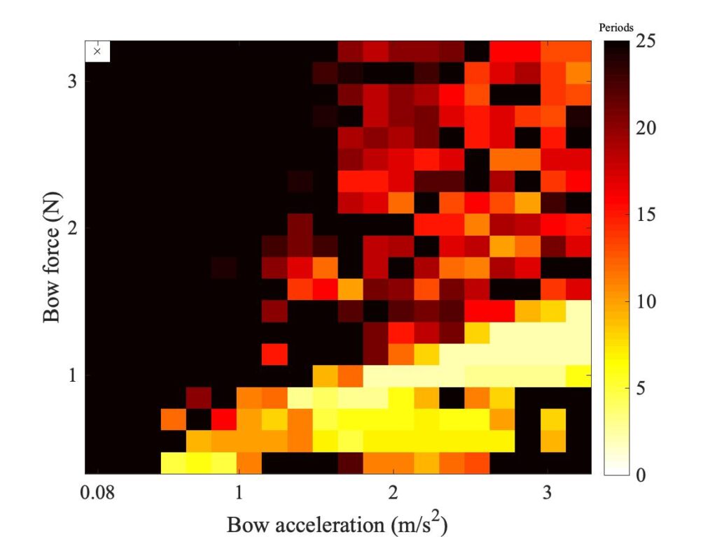
We don’t exactly see convergence in this sequence of plots, but we didn’t really expect to — we have already seen several examples of bowed string transients showing sensitive dependence, so any small change is likely to make a difference to individual “speckles” in the pattern. But at a more qualitative level, the story told by Fig. 2 is quite encouraging. Even with 2 “hairs”, the region containing coloured pixels grows to a size comparable with the Galluzzo measurement (shown below in the first panel of Fig. 3). Adding more “hairs” changes the details, but the broad pattern remains very stable. The core region of the shortest transients remains very similar throughout the sequence.
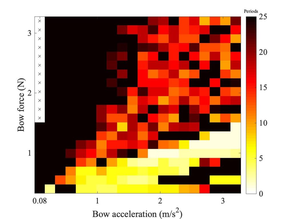
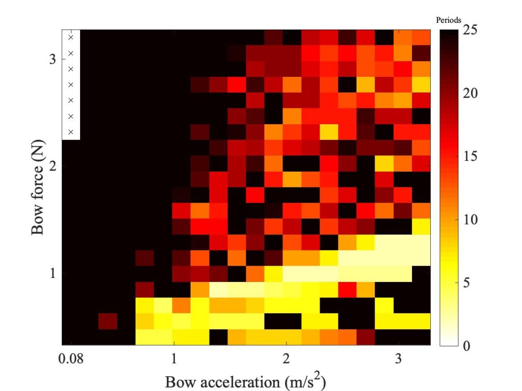
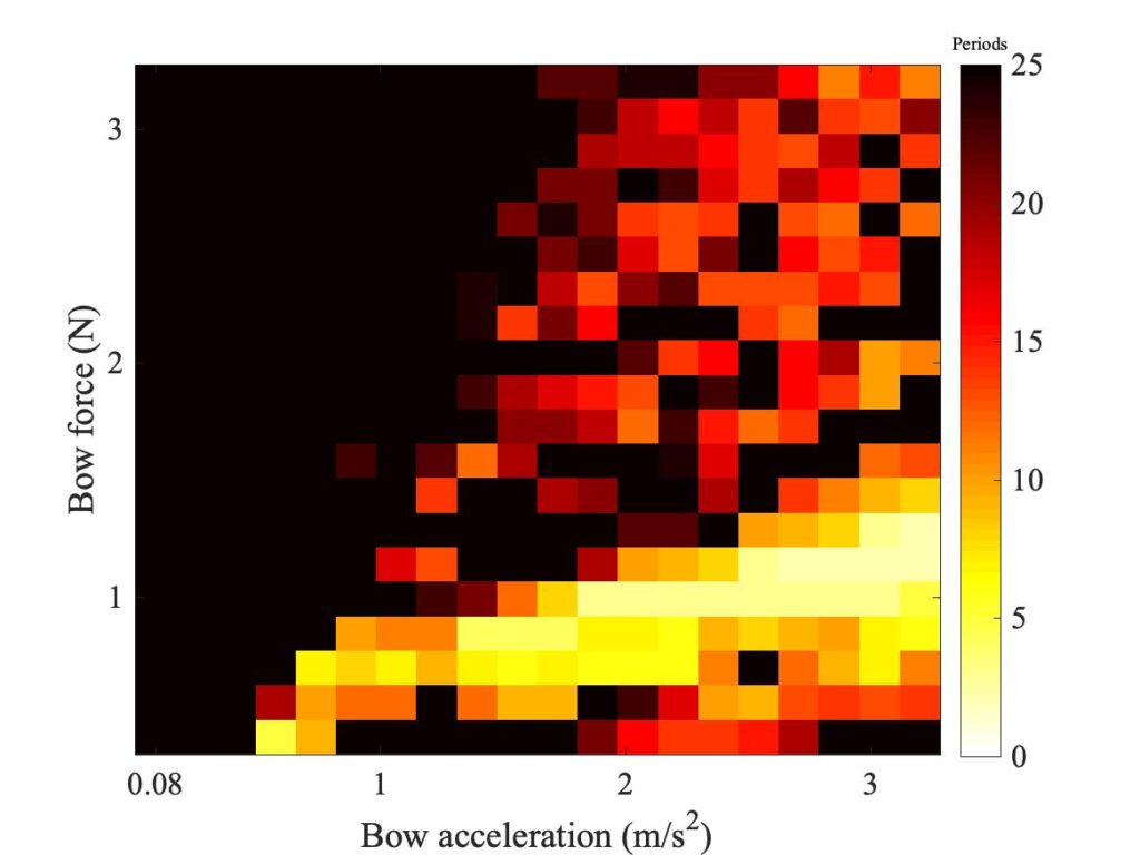
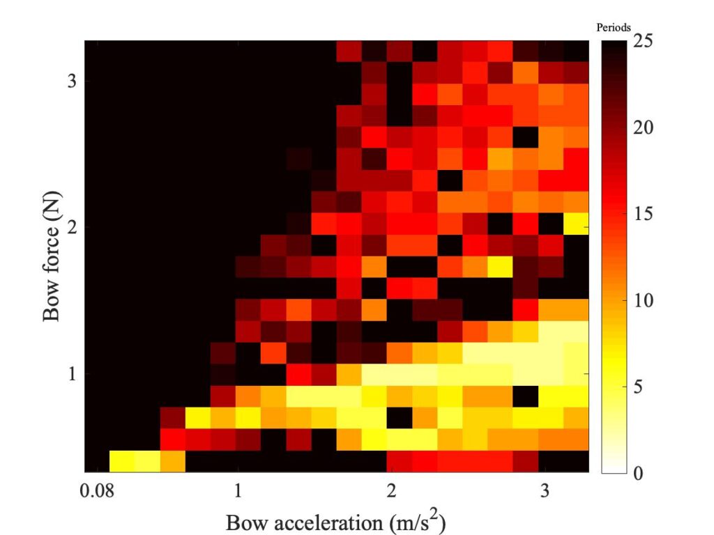
The next step is to look at the effect of changing the friction model. It was found that simulations using the friction curve model gave results that were so distant from the measurements that it is not worth discussing them in any detail. But the two thermal models both gave plausible results. Figure 3 shows the same Guettler diagram, simulated using 6 “hairs”, using both models. The top panel shows the measurement, the middle one shows simulated results with the original thermal model, and the lower panel (a repeat of the last panel of Fig. 2) shows results with the enhanced thermal model.
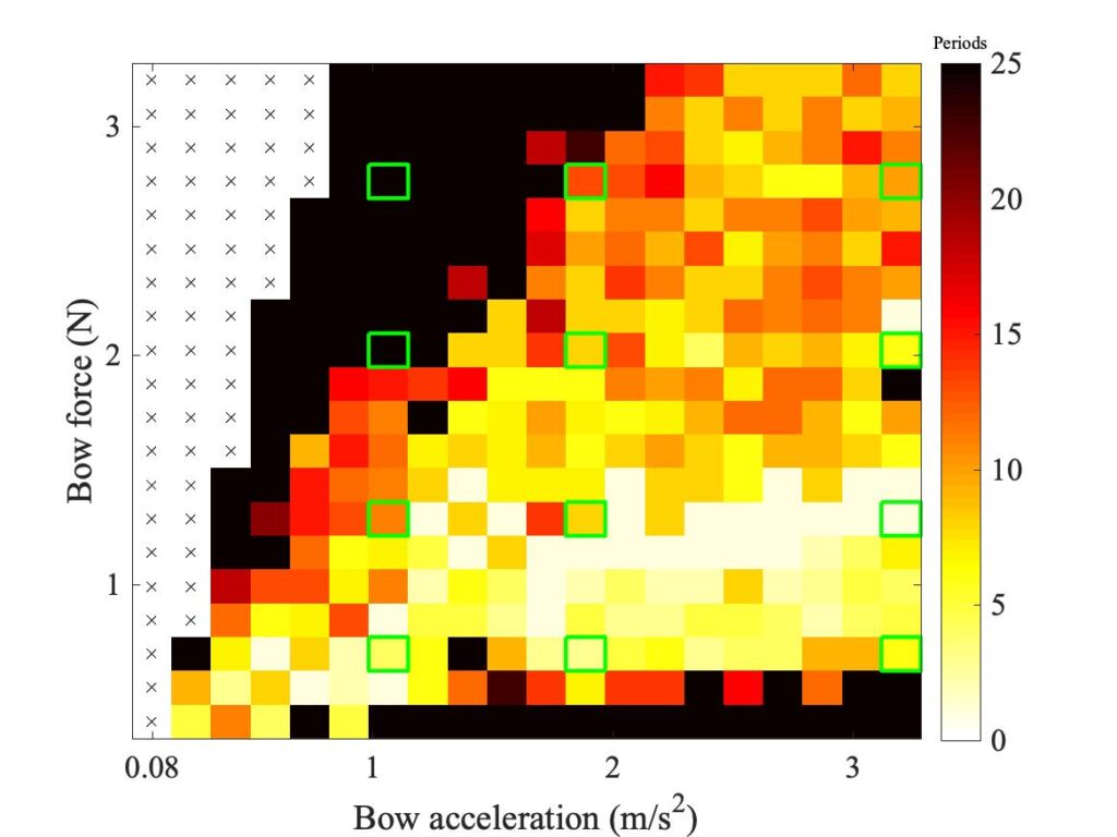
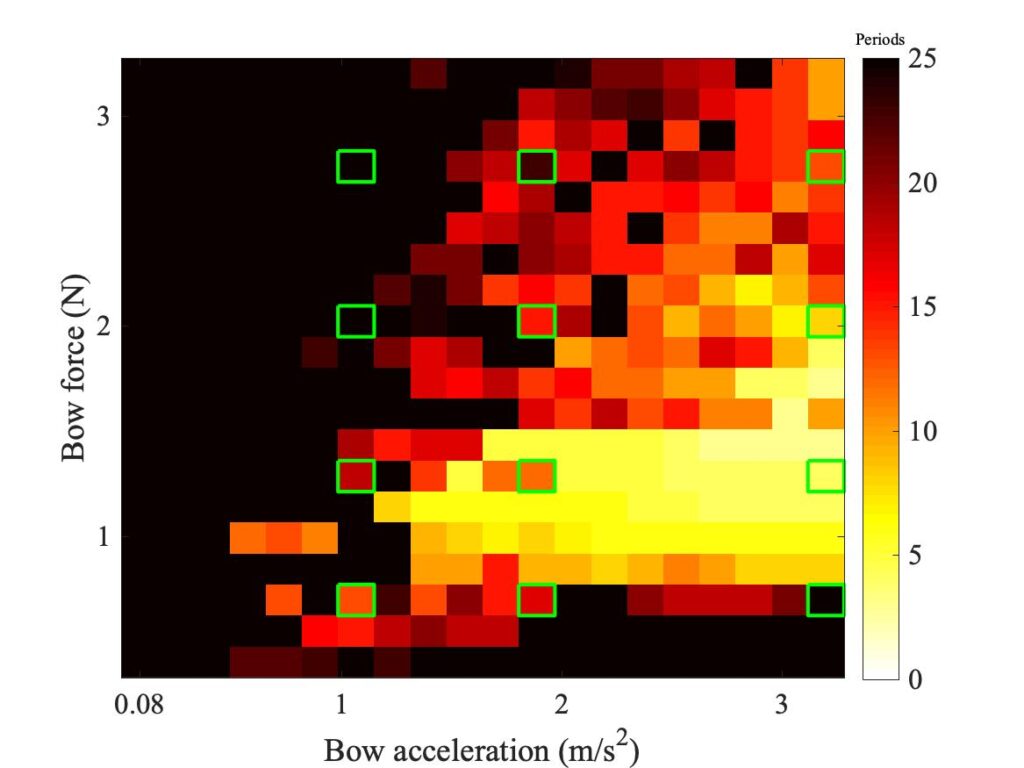

Neither simulation model entirely captures all elements of the measurement. Both show the correct broad distribution of coloured pixels, although neither model populates the lower left-hand corner of the plot as much as the measurement requires. The enhanced model perhaps does slightly better in this regard, since at least it shows a small wedge of coloured pixels reaching almost to the corner of the plot. On the other hand, the enhanced model falls down a little by showing a band of dark pixels slanting upwards across the lower half of the plot, while there is no trace of such a feature in the measurement or in the other simulation.
To see a little of what lies behind these Guettler plots, all three panels of Fig. 3 are annotated with a grid of green squares, marking cases that are examined in more detail in Figs. 4—7. Each of these figures corresponds to one row of the green squares, with three panels corresponding to the left, middle and right square of the row. Each individual panel shows 5 bridge-force waveforms. At the top in black is the measurement, corresponding to the top panel of Fig. 3. In red is the finite-width simulation using the original thermal model, and below it in magenta is the corresponding point-bow simulation. In blue is the finite-width simulation using the enhanced thermal model, and in green the corresponding point-bow simulation.
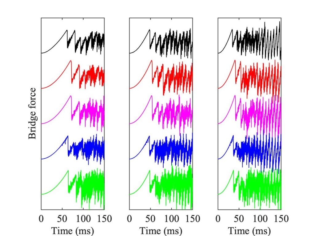
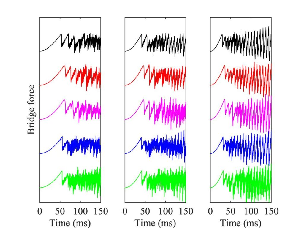
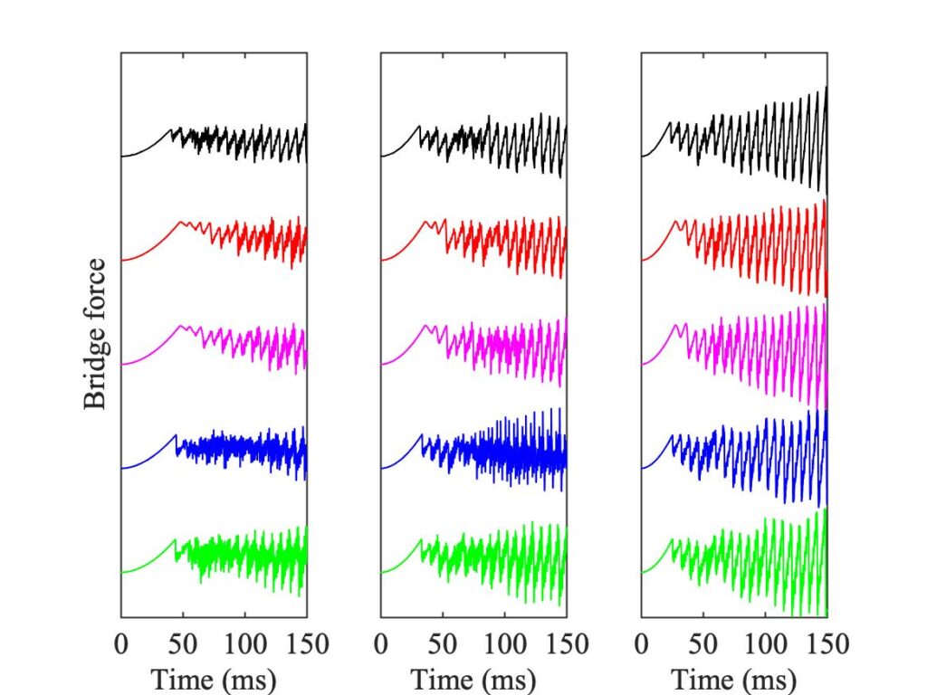
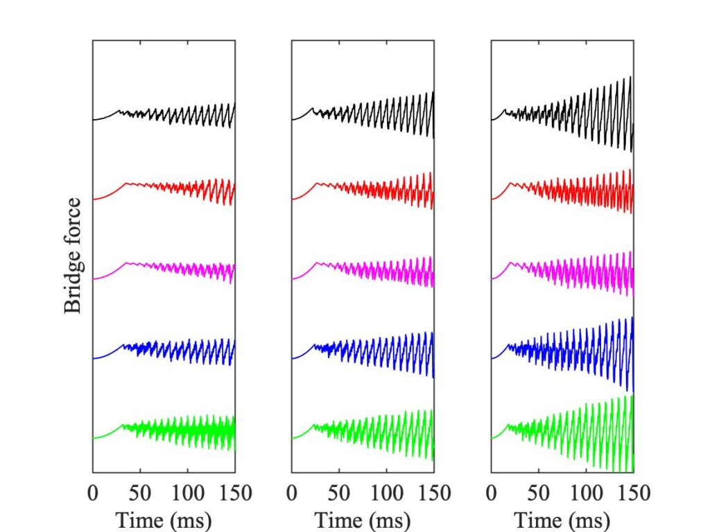
Many details can be seen by careful study of these plots. They confirm that none of the simulation models gives a perfect match to the measurements, but that on the whole finite-width simulations do a better job than point-bow simulations, and that in at least some respects, the enhanced thermal model does better than the original model. Always we need to keep in mind the phenomenon of sensitive dependence. It is a great pity that we do not have nominally identical repeat tests for the experimental results, to illustrate that fact directly.
[1] R. Pitteroff and J. Woodhouse, “Mechanics of the contact area between a violin bow and a string. Part II: simulating the bowed string”; Acta Acustica united with Acustica, 84, 744—757 (1998).
[2] R. Pitteroff and J. Woodhouse, “Mechanics of the contact area between a violin bow and a string. Part I: reflection and transmission behaviour”; Acta Acustica united with Acustica, 84, 543—562 (1998).
[3] Hossein Mansour, Jim Woodhouse and Gary P. Scavone, “Enhanced wave-based modelling of musical strings, Part 1 Plucked strings”; Acta Acustica united with Acustica, 102, 1082–1093 (2016).