
We did not need to think about torsional motion when we looked at plucked strings, but in a bowed string torsion can play a significant role. The first step is to derive the differential equation governing small-amplitude torsional motion in a string (or indeed in any other system, such as the shaft of an engine). As we have done several times before, we look at the forces acting on a small element of the string, as sketched in Fig. 1. We assume the string has external radius $a$, and has rotational displacement $\theta(x,t)$ driven by an external torque $M(x,t)$ per unit length. We start by thinking of a string made of a single material, with density $\rho$ and shear modulus $G$.
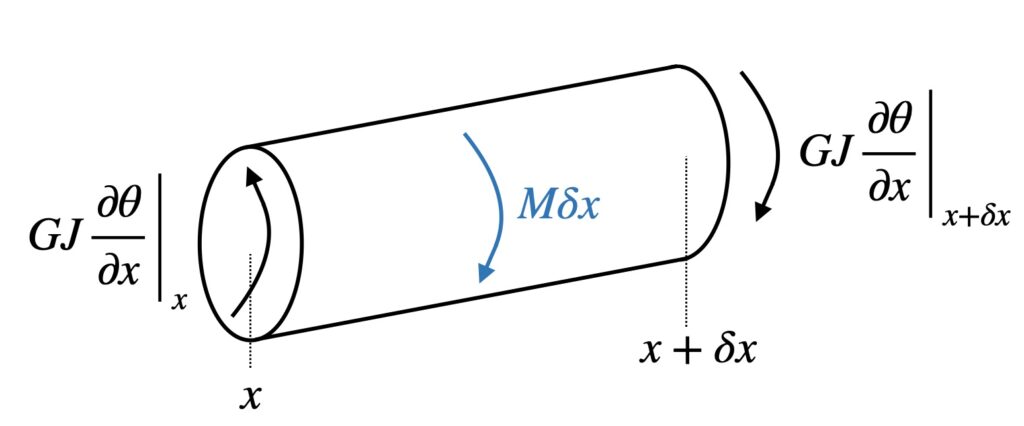
At each end of the element, there is a torque associated with the local deformation, which is resisted by the shear rigidity of the material. This torque takes the form $GJ \dfrac{\partial \theta}{\partial x}$, a form that is completely analogous to the force $T \dfrac{\partial w}{\partial x}$ associated with transverse displacement $w(x,t)$ of a string under tension $T$, as we saw in section 3.1.1. $J$ is the polar moment of area per unit length, which for a uniform circular string is given by
$$J=\dfrac{\pi a^4}{2} . \tag{1}$$
For our string element, we have this torque acting at both ends, while the external torque contributes $M \delta x$. The rotational version of Newton’s law then gives
$$I \delta x \dfrac{\partial^2 \theta}{\partial t^2} = M \delta x +GJ\left[ \left.\dfrac{\partial \theta}{\partial x} \right|_{x+ \delta x} -\left.\dfrac{\partial \theta}{\partial x} \right|_{x} \right] \tag{2}$$
where $I$ is the polar moment of inertia per unit length, given by $I=\rho J$ for a uniform string.
In the limit $\delta x \rightarrow 0$, this gives us the governing equation
$$I \dfrac{\partial^2 \theta}{\partial t^2} – GJ \dfrac{\partial^2 \theta}{\partial x^2}= M . \tag{3}$$
For the uniform string, the factor $J$ cancels out, leaving
$$\rho \dfrac{\partial^2 \theta}{\partial t^2} – G \dfrac{\partial^2 \theta}{\partial x^2}= M . \tag{4}$$
This is the one-dimensional wave equation, with exactly the same form as we found for the ideal string (section 3.1.1) and for plane sound waves (section 4.1.1). The only difference between those three cases comes in the particular constants: $G$ and $\rho$ in this case. The wave speed is given by
$$c_t=\sqrt{G/\rho}. \tag{5}$$
This is the shear wave speed of the material, dependent on the material properties but independent of the radius of the string. However, for a typical musical string with a complicated construction involving multiple layers of material, the parameter $GJ$ is best regarded as an effective property of the string, determined by measurement or more detailed modelling. The torsional wave speed is then $c_t=\sqrt{\dfrac{GJ}{I}}$. The polar moment of inertia $I$ can be calculated straightforwardly if the thickness and density of each layer is known since it is defined by
$$I= 2 \pi \int_0^a{r^3 \rho(r) dr} . \tag{6}$$
Because torsional waves obey the same equation as transverse waves on an ideal string, many results we have already seen relating to transverse vibration have direct counterparts for torsion. One important example relates to impedance. Consider the excitation of torsional motion by a force $fe^{i \omega t}$ applied on the surface of the string. The corresponding moment is $afe^{i \omega t}$. This will generate string rotation $\theta$, which in turn produces surface displacement equal to $a \theta$.
The point force will generate outgoing torsional waves at the frequency $\omega$, symmetrically in the two directions. We can write these in the form
$$\theta(x,t)= A e^{i \omega t \pm i k x} \tag{7}$$
where the $\pm$ signs apply to the two directions of travel, $A$ is an amplitude factor, and $k=\omega /c_t$ is the wavenumber for torsional waves. There will be a jump in $\dfrac{\partial \theta}{\partial x}$ at the point where the force is applied, which we can take to be $x=0$. Moment balance at that point then requires
$$fa=2 G J A i k \tag{8}$$
so that the surface velocity is
$$v = i \omega a A = i \omega a \dfrac{fa}{2GJ i \omega /c_t}=\dfrac{f a^2 c_t}{2GJ}=\dfrac{fa^2}{2 \sqrt{GJI}} . \tag{9}$$
The ratio of force to velocity is independent of frequency $\omega$: torsion on an infinite string behaves like a dashpot, just as we saw for transverse vibration of an ideal string. That ratio is
$$\dfrac{f}{v}=\dfrac{2 \sqrt{GJI}}{a^2} \tag{10}$$
and for the case of a uniform string this reduces to
$$\dfrac{f}{v}=\dfrac{2 J\sqrt{G\rho}}{a^2}=\dfrac{2}{a^2}~\dfrac{\pi a^4}{2} \sqrt{G \rho}=\pi a^2 \sqrt{G\rho} . \tag{11}$$
The corresponding result for transverse motion was $2 Z_0$ in terms of the string impedance $Z_0=\sqrt{T m}$ where $T$ was the tension and $m$ the mass per unit length, so we see that the torsional quantity corresponding to $Z_0$ is
$$Z_t=\dfrac{\sqrt{GJI}}{a^2}=\dfrac{\pi a^2}{2} \sqrt{G\rho} \tag{12}$$
where the first expression is for the general case, and the second for the case of a uniform string.
On an infinite string, the tangential force $f$ would result in surface motion from both transverse and torsional motion, and the combined motion would be the sum of these. That means that such combined motion would be governed by a parallel combination of the two impedances, with a combined value $Z_{eff}$ satisfying
$$\dfrac{1}{Z_{eff}}=\dfrac{1}{Z_0}+\dfrac{1}{Z_t} . \tag{13}$$
The two impedances $Z_0$ and $Z_t$ play a role in the final topic to be examined here. Back in section 9.2 we saw the origin of the pattern of Schelleng ripples, sketched in Fig. 13 of that section. Each time the rounded Helmholtz corner passed the bow, it generated perturbations on the string, reflected back from the bowed point. These then travelled up and down on the string, and when they encountered the sticking bow they were totally reflected from it.
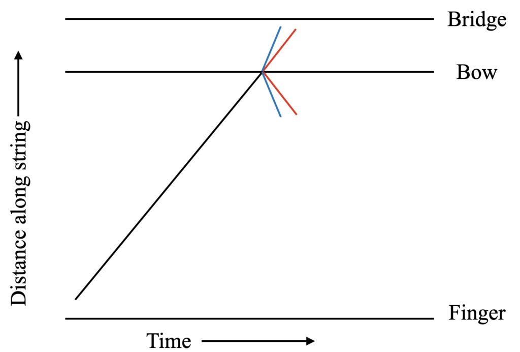
Once we include the possibility of torsional motion, that simple picture changes. Now when a velocity perturbation reaches the sticking bow, it can cause motion even though sticking is not interrupted, because the string can roll on the bow. Rolling consists of equal and opposite components of surface motion associated with transverse and torsional waves, so that the sum of the two gives zero velocity relative to the bow. This is, of course, the condition for sticking.
The situation is then as sketched in Fig. 2. The incident transverse wave, shown in black, produces four separate outgoing waves: transmitted and reflected transverse waves, shown in red, and transmitted and reflected torsional waves, shown in blue. The torsional waves generally travel faster than the transverse waves. For the case of an ideal flexible string without bending stiffness, the reflection and transmission coefficients for all four of these waves are determined completely by the ratio $Z_0/Z_t$. We needn’t go through the details: they can be found in reference [1], together with the more complicated results when allowance is made for bending stiffness, and also for compliant behaviour of the bow.
[1] R. Pitteroff and J. Woodhouse, “Mechanics of the contact area between a violin bow and a string. Part I: reflection and transmission behaviour”; Acta Acustica united with Acustica, 84, 543—562 (1998).