To get the most accurate estimate of a bridge admittance, or any other frequency response function of a linear system, it is advisable to make multiple measurements and use some form of averaging. We are dealing with a system like the sketch below, reproduced from section 2.1. (Of course, the system we are measuring is not necessarily a drum!)

Suppose we have an input signal $x(t)$ and an output signal $y(t)$. We can call their Fourier transforms $X(\omega)$ and $Y(\omega)$. If we could take measurements for infinite time, with no contamination by noise, and if our system really was perfectly linear, then the frequency response we want is simply the ratio $Y(\omega)/X(\omega)$. But none of those things will be true in a real measurement. We catch a finite chunk of the input and output signals, and use the FFT to convert them to the frequency domain. The ratio of these will indeed give us an estimate of the frequency response function, but for mathematical reasons that we will not go into here, simply repeating that process several times and taking the average of these individual estimates of the complex response is not the best thing to do.
A better approach makes use of concepts from the field of random vibration, concerned with questions like describing the vibration response of an offshore oil platform exposed to ocean waves, or the noise inside a car as a result of tyre noise from the rough surface of the road. We can define something called the power spectral density of the input
$$S_{xx}(\omega) = \frac{1}{T}\left<|X(\omega)|^2 \right> = \frac{1}{T}\left<X(\omega) X^*(\omega)\right> \tag{1}$$
where $T$ is the length of the chunk of signal that has been processed, $X^*$ denotes the complex conjugate of $X$, and $\left< … \right>$ means ‘average value over the multiple measurements’. Similarly, we define
$$S_{yy}(\omega) = \frac{1}{T}\left<Y(\omega) Y^*(\omega)\right> .\tag{2}$$
Finally, a related quantity is the cross spectral density of the output and input:
$$S_{xy}(\omega) = \frac{1}{T}\left<X(\omega) Y^*(\omega)\right> .\tag{3}$$
Given these three averaged quantities, there are two different ways that we might estimate the thing we really want, $Y/X$: either as $S_{yy}/S_{xy}$, or as $S^*_{xy}/S_{xx}$. If everything is working perfectly, these two estimates should be equal. A useful measure of whether this is happening is the coherence function $C_{xy}$ defined as the ratio of the two:
$$C_{xy}(\omega)=\dfrac{S_{xy}(\omega)S^*_{xy}(\omega)}{S_{xx}(\omega) S_{yy}(\omega)} .\tag{4}$$
Since the two power spectral densities are by definition real and positive, and the expression in the numerator is $|S_{xy}(\omega)|^2$, it is obvious that this is a positive, real quantity, not a complex one. It always lies between 0 and 1.
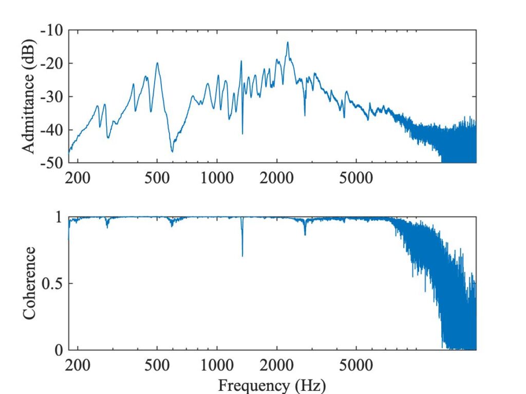
An example is shown in Fig. 2: this is a rather good-quality measurement, showing coherence close to 1 up to about 7 kHz. In that range, where the coherence is seen to drop a little it can be seen to correspond to frequencies where the admittance was low, so that the signal-to-noise ratio of the measurement was relatively poor. However, this plot is deliberately shown over an extended frequency range, up to 20 kHz. The impulse hammer hitting the wood of a violin bridge does not supply reliable input at these higher frequencies, and the coherence falls off dramatically. The coherence function thus gives an immediate impression of the effective bandwidth of the measurement.