
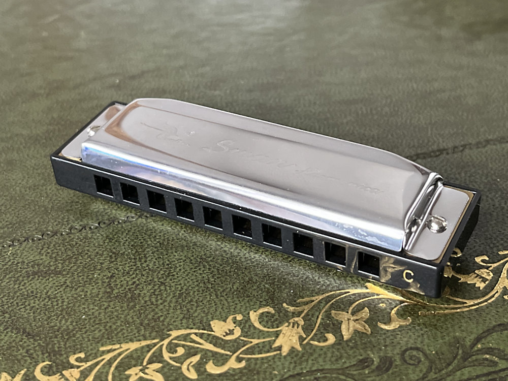
We now turn to the next family of wind instruments, the “free reeds”: this family includes the harmonium, the accordion, the concertina and the harmonica. We can illustrate the shared features of these instruments with a harmonica. Figure 1 shows a typical 10-hole diatonic harmonica; first in its complete state, and then after the cover plates have been removed. The central “comb” creates a series of small chambers into which the player can blow or suck air. Each of these chambers aligns with two thin brass reeds, fixed over slots in the two reed plates. One set of reeds, shown in close-up in the lower left-hand image, are fixed to the inner surface of the plate, while the other set (shown on the right) are fixed to the outer surface. A reed from the first set will vibrate when the player blows into the corresponding hole: these are the “blow reeds”. The second set are called the “draw reeds”, and are ordinarily set into vibration by sucking air out of the hole.


A harmonium or reed organ has only “blow reeds”: air always flows in one direction, pumped by hand, or foot pedals, or an electric pump. However, instruments like the concertina, accordion or bandoneon have sets of inward-facing and outward-facing reeds similar to the harmonica. The air flow is created by the player expanding or compressing a bellows-like structure. Buttons or keys are used to operate levers which open internal valves to allow the air to flow into or out of each reed chamber. Figure 2 shows a concertina, disassembled into some of its component parts. On the lower right, the radial reed chambers can be seen. In each chamber one reed is visible, while another is on the reverse side of the plate, hidden from view by a leather flap which reduces air leakage when the first reed is being played.

What all these instruments lack, in contrast to the reed and brass instruments discussed in earlier sections, is any kind of resonating tube to determine the playing pitch. Instead, the pitch is determined by the lowest vibration resonance of the reed itself. But it is not immediately clear why air-flow past a reed should set it into vibration, nor why vibration only occurs when the air-flow is in one direction through the reed plate, and not in the reverse direction. Why do blow reeds only blow, and draw reeds only draw?
These are questions we want to address by modelling and simulation, but we will discover that the answers are complicated, and not fully understood yet — we will come up against a frontier of research. In summary, it currently looks as if there may be two different mechanisms of instability of free reeds: one related to the kind of effects we have been talking about in the previous sections on reed and brass instruments (and therefore amenable to a similar style of modelling), the other involving more challenging fluid dynamical effects that are harder to model in a simple way. Of course, for something like the concertina shown in Fig. 2, part of the answer seems simple: the leather flaps prevent significant air flow in the reverse direction, so the question of which reed sounds for a given direction of air-flow doesn’t really arise. But there is more to the question than that, as we shall see.
The first step towards addressing this question seems paradoxical. There is very little scientific literature on the theory of free reed vibration, and there has apparently been only one careful experiment designed to test the predictions of a theory in quantitative detail (by Tarnopolsky, Fletcher and Lai [1]). But that experiment makes use of a test system in which what looks like a draw reed in fact chooses to vibrate as a blow reed! We will come to the details of their model and experiment shortly, but it gives an immediate hint that the answer to the question we just asked might be rather subtle and complicated.
The key difference between the two reed configurations is sketched in Fig. 3. On the left, the reed is attached to the plate on the same side as the source of air flow. That means that if the reed displaces slightly in the direction of the air flow, it tends to reduce the area of gap between the reed and the plate: a “closing reed”. On the right, the reed is attached on the opposite side of the plate and if it moves in the direction of the air flow the gap increases: an “opening reed”. We can recognise both these tendencies from earlier sections: reed woodwind instruments like clarinets and saxophones have closing reeds, while our model for a brass-player’s lip buzzing was an opening reed.

We have already seen that the minus sign needed to turn a closing reed model into an opening reed model had profound consequences for the behaviour of those instruments. A similar profound difference applies to free reeds. All the free-reed instruments we have mentioned are designed to play with closing reeds, as we can see in the two pictures in the bottom row of Fig. 1: the blow reeds, on the left, are inside the cavity, while the draw reeds on the right are outside the cavity. A given reed cannot ordinarily be made to vibrate by air flow in the “opening reed” direction, and this is vital to the normal functioning of the instrument: you expect to get a different note when blowing or drawing on a given reed cavity.
It is time to think about developing a theoretical model for free-reed instruments. You might think that the simplest model would correspond to a reed set in a wall between two large open spaces, with a different steady pressure imposed in the two spaces. That would certainly create some air flow past the reed, related to the pressure difference by the kind of model we have already used successfully for woodwind and brass instruments.
But this configuration lacks a crucial ingredient if we want to build a model like the earlier ones. In our models of woodwind and brass instruments, spontaneous oscillation happened as a result of a feedback loop, in which the air flow past the reed interacted with the acoustical response of the instrument tube. But if both sides of the reed are essentially open to empty space, no such strong acoustical feedback can occur. That is not to say that a reed set in a wall between two large rooms might not vibrate with sufficient pressure difference — it almost certainly could if the geometrical details around the reed were suitably designed. But such a spontaneous vibration would rely on a different kind of instability, depending on the detailed pattern of local fluid flow. We will side-step this possibility for the moment, but we will return to it later, at least briefly.
The very simplest option to create some acoustic feedback is to have the reed set in the wall of a closed chamber with a finite volume. Air flow in and out of this chamber will automatically create changes of mean density, leading to changes of pressure that can provide acoustical feedback on the reed vibration. In terms of instruments, this chamber might correspond to the bellows of a concertina or the mouth cavity of a harmonica player. The resulting idealised geometry is sketched in Fig. 4, and this is precisely the situation investigated by the experiment of Tarnopolsky, Fletcher and Lai [1], designed to test a theoretical model developed earlier by Fletcher [2].

Fletcher’s analysis, as applied to this configuration, is described in the next link. He used linearised theory to investigate the threshold of instability in terms of the mean pressure inside the volume (which in turn is determined by the rate of air-flow injected into the volume by the player). Before we see some results of his predictions, we need to understand a feature of free reeds which distinguishes them from clarinet reeds or brass player’s lips. When the reed moves towards the slot in the reed plate, it initially reduces the gap as we have already said. But the reed does not close the gap completely: instead, the reed can pass right through the gap and move out on the other side as sketched in Fig. 5.

Our model for air-flow through the reed (see section 11.3.1) involves the area of the gap, as a function of the tip displacement of the reed. For the opening-reed configuration shown in Fig. 4, that area function looks like the red curve in Fig. 6. For a positive tip displacement (away from the wall of the chamber, in the opening-reed direction), the area simply increases with displacement. But for a negative displacement the area reduces initially, then is roughly constant when the reed lies within the thickness of the plate, then increases again once the reed comes out on the other side so that the gap starts to grow. If the same reed were swapped around to the closing-reed configuration, the result would be the blue curve in Fig. 6. This is simply the reflection of the red curve in the vertical axis.

Putting these ingredients together, Fletcher predicted that the reed would vibrate most readily in the opening-reed orientation. He then predicted that the threshold pressure would depend on the volume of the cavity, and also on the Q-factor of the reed vibration. These are the predictions that were tested in the experiment by Tarnopolsky, Fletcher and Lai. Their results are summarised in Fig. 7. The four lines show the predicted pressure threshold as a function of volume, for four different values of the Q-factor. The stars in corresponding colours show the measured results. It is immediately clear that the agreement is not perfect, but that the qualitative trends were matched and the quantitative agreement is pretty good (they did not give estimates of their experimental uncertainties).

This leaves us with the paradox mentioned earlier. Why does this configuration of reed and chamber mean that the reed prefers to vibrate in the opening-reed orientation, when all free-reed instruments do the opposite? We can shed some light on this question by enhancing the model in a very simple way suggested by Millot and Baumann [3] and sketched in Fig. 8. Instead of connecting directly to the wall of the chamber, the reed is driven via a small tube. As explained in the next link, this makes a small but crucial difference to the stability analysis. One extra parameter now enters: the Helmholtz resonance frequency of chamber and tube, when the reed is absent and the tube is open at the right-hand end.

The behaviour then depends on whether that Helmholtz resonance frequency is above or below the resonance frequency of the reed: a crucial sign is reversed by this choice, and this interacts with another important sign associated with the area function from Fig. 6. Figure 9 shows a version of that area function relevant to the geometry of the Tarnopolsky, Fletcher and Lai experiment, except that for reasons to be explained shortly I have set the thickness of the reed plate to 1 mm rather than the actual 4 mm. The only aspect of these curves that enters the stability analysis is the slope — but this is not the slope near zero displacement, it is the slope at the “operating point” of the reed. The static blowing pressure means that the reed is displaced outwards. The four vertical dashed lines in the plot show the displacements corresponding to zero pressure (on the left), and to 1, 2 and 3 kPa moving progressively rightwards.

Now look at the slopes of the red and blue curves where these dashed lines cross them. For the opening reed (red curve), the slope stays positive throughout, and indeed it hardly changes as the operating point shifts. But the blue curve shows more complicated behaviour. Initially, the slope is strongly negative. Once the pressure reaches about 1 kPa, the reed has moved inwards far enough to compensate for the 1 mm stand-off from the reed plate, so the reed enters the slot in the plate and the slope begins to level off. Once the pressure gets above about 2 kPa, the reed tip starts to emerge on the other side of the plate, and the slope reverses. By 3 kPa the reed has moved well beyond the plate, and the slope is positive, not very much lower than the slope of the red curve. It was in order to reach this final state with a reasonable mouth pressure that I chose to reduce the plate thickness to 1 mm.
Now we can look at the behaviour of the threshold blowing pressure, and Fig. 9 will help us to understand the results. Some cases are illustrated in Figs. 10 and 11. The Q-factor of the reed is kept fixed at 55, while we vary the frequency ratio of the reed resonance to the Helmholtz resonance. In Fig. 10 the Helmholtz resonance is always higher than the reed resonance. The solid red curve shows the threshold for the opening reed when the Helmholtz resonance frequency is very high. This curve is essentially identical to the black curve in Fig. 7 (it only looks different because the plotting ranges are different in the two figures).

The explanation lies in the comparison of Figs. 4 and 8. The original Fletcher case of Fig. 4 is a special case of Millot’s model in Fig. 8, in which the length of the extra tube has been shrunk to zero. That has the effect of sending the Helmholtz resonance frequency off towards infinity, so that it is much higher than the reed resonance frequency. The other solid curves in Fig. 10 show what happens as the Helmholtz resonance frequency comes down, until it is only 5% higher than the reed resonance (black curve). The opening-reed configuration plays more and more easily!
The dash-dot curves in Fig. 10 show the corresponding pressure thresholds for the closing-reed configuration. For all four curves, the closing reed can indeed be induced to vibrate, with a pressure above 2 kPa. Figure 9 explains what is happening: we already commented that above about 2 kPa, the slope of the blue curve for the closing reed reverses, so that it has the same sign as the red curve. That slope is the only thing that enters the stability calculation, so we should not be too surprised to see Fig. 10 predicting instability of the closing reed at this kind of pressure.
Figure 11 shows the corresponding plot for several cases in which the Helmholtz resonance frequency is lower than the reed resonance frequency. The behaviour has reversed: we only see dash-dot curves. The closing-reed configuration is now the one that plays quite readily, and the opening-reed case never plays. This is the pattern we expect from all the free-reed instruments we looked at earlier. Notice that the pattern is also consistent with what we found in earlier sections: the brass instruments, with a opening-reed configuration, always have a playing frequency above the “reed” resonance, whereas the reed woodwinds, with a closing-reed configuration, typically play at frequencies well below the reed resonance.

Insofar as Millot’s model can be applied to real instruments, these results suggest that with any free-reed instrument featuring pairs of opening and closing reeds, we should always expect one reed to function as a draw reed and the other as a blow reed. But they could be either way round: which is the blow reed and which is the draw reed depends on the resonance frequencies of the reeds relative to the Helmholtz resonance frequency of the instrument.
This raises an obvious question: why does it seem to be the case that all normal free-reed instruments operate in the closing-reed configuration? We can get some insight into that question from Fletcher’s original analysis, which was couched in terms of impedance. Some details were given at the end of the first side link above. The analysis shows that instability depends crucially on the sign of the imaginary part of the impedance: that sign must be positive at the oscillation frequency of a closing reed, or negative for an opening reed. But this brings us to the frontier of current knowledge. Can Millot’s model really be applied to real instruments? And if so, why do they all show a pattern with the imaginary part of the impedance positive? To go further, what is needed is some measurements of input impedance in free-reed instruments — a promising future topic for researchers in the field.
It is prudent, and also of interest in its own right, to check the predictions of the linearised stability theory against the results of simulations. For this purpose we will not use the rather unusual reed geometry of the Tarnopolsky experiment, but instead we will apply Millot’s model to a typical harmonica reed. We expect a harmonica reed to play in a closing-reed configuration, so the Helmholtz resonance frequency was chosen to be lower than the reed resonance by a factor 1.5. Running a grid of simulations for various values of cavity volume and mouth pressure, we obtain results as shown in Figs. 12 and 13. Figure 12 is colour-shaded to indicate the spectral centroid of the waveform of pressure inside the reed chamber, while Fig. 13 shows the peak-to-peak amplitude of that pressure waveform.


It is immediately apparent from Fig. 12 that the simulation results agree very well with the predicted stability threshold, shown in the blue curve. It is not so easy to see this agreement in Fig. 13, however, because the amplitude of the pressure signal fades away as the cavity volume increases. To see what this means in terms of the pressure waveforms, Fig. 14 shows the final periodic portion of the five cases marked by a green rectangle in Figs. 12 and 13. You can listen to these five synthesised waveforms in Sound 1: it is obvious that the sound gets progressively quieter as the cavity volume increases. We should not be surprised by this: we introduced the finite cavity volume in order to provide acoustical feedback to the reed, but the bigger the cavity the weaker that feedback will be because a given amount of airflow induced by the reed motion will have less impact on the pressure in a larger chamber.

The pressure waveforms revealed in Fig. 14 show a pair of peaks in every cycle. To see how these arise, Fig. 15 shows one of these waveforms alongside other quantities that are computed in the course of the simulation. The top curve shows the displacement of the reed tip. The dashed lines mark the thickness of the reed plate: I have deliberately chosen a rather extreme case, in which the reed vibrates through the plate and out on the other side. The second panel of Fig. 15 shows the pressure waveform we have already seen (it is the top one in Fig. 14); the third panel shows the rate of air flow past the reed. Comparing these with the top panel, it is clear that each time the reed tip passes through the plate, obstructing the gap through which air can flow, there is strong dip in the air flow rate, and a big peak in the pressure inside the reed cavity. The reed motion looks more or less sinusoidal, but the “peaky” pressure waveform is very rich in higher harmonics, a characteristic feature of the sound of free-reed instruments.

Figure 16 shows the initial transient from one of the simulations — specifically, it corresponds to the second pixel from the left in the marked rectangles in Figs. 12 and 13. The early part of the transient shows a single pressure peak in each cycle, because the reed is not yet passing right through the plate. But as the amplitude grows, the second peak builds up until it is roughly half the height of the first peak, as we saw in the final periodic waveform (second from the top in Fig. 14).

I said we would return briefly to the question of whether there might be an alternative source of instability of a free reed in a flow. An idealised problem we mentioned at the beginning is that of a reed set in a partition between two anechoic rooms. No model of the kind we have looked at can then be formulated consistently: the pressure is simply constant (but different) on the two faces of the reed and there is no predicted instability. However, it is possible that there is some purely fluid-dynamical mechanism, not relying on acoustic feedback, that can predict instability.
A suggestion along these lines has been advanced by Ricot, Caussé and Misdariis [4]. They consider the flow pattern in the vicinity of a reed, but their model involves non-trivial fluid dynamics and so in order to make progress with the analysis they were forced to use a highly idealised version of the geometry of the reed and its slot. When they solved their model numerically, they did indeed find that it predicted oscillation of a closing reed. The success of Tarnopolsky, Fletcher and Lai [1] in matching experiment with the acoustic feedback theory in an opening-reed configuration suggests that when strong acoustic feedback is present, it can be dominant under at least some circumstances. But it seems likely that the fluid-dynamical instability mechanism is also present, producing a bias in favour of closing reeds which plays a significant role in the behaviour of many free-reed instruments.
We can show some direct evidence relating to the two different instability mechanisms. Figure 17 shows the apparatus for a partial re-run of the experiment by Tarnopolsky et al. [1]. The very wide reed can be seen at the front, and behind it is a cylindrical chamber whose volume can be varied by moving a piston. Air flow is delivered by a pipe in the middle of this piston. In this version of the experiment the air is sucked rather than blown from the pipe, so the arrangement of the reed on the inner face of the front plate means that it is in the opening configuration. A microphone is placed in the side wall of the chamber to record the internal sound pressure, and a small clear tube leads to a pressure sensor to measure the static pressure difference from the outside world.
Figure 18 shows some results, in a similar format to Fig. 7. For a few values of the internal pressure, the volume was varied by moving the piston in small steps. The black stars mark the cases where a sound could be heard from the reed. The symbol sizes have been scaled so that their areas are proportional to the peak-to-peak amplitude of the sound pressure measured inside the chamber by the microphone. The red curve shows the threshold predicted by Fletcher’s theory, with parameter values appropriate to this experiment. The Q-factor of the reed was quite high, around 250, so the threshold pressure is lower than in any of the cases shown in Fig. 7. The rather jagged coloured lines show a contour map of the predicted peak-to-peak pressure, computed from a $50 \times 50$ grid of simulations using the model described above.

It can be seen that the experimental results agree well with some aspects of the predictions, but not all. The threshold line in the left section of the plot is matched very well. The qualitative trend of peak-to-peak sound pressure is also followed, with the highest values found just above the threshold and concentrated in the upper left-hand portion of the plot. However, with larger cavity volumes the measurements show a cessation of noise above about 2.5 l volume, but the model prediction is that the reed should remain unstable across the entire width of the plotted region, albeit with an amplitude that is quite low. So something is wrong with the model in this region, but the precise explanation is not known. There are many possibilities; both among the idealisations used to formulate the simple model, and among the details of the experimental apparatus.
But there is another experimental result to be reported from this apparatus. At the end of the testing sequence to give the points in Fig. 18, the front plate holding the reed was removed and turned round, so that the reed was in the closing configuration. According to the Fletcher model, the pressure should then have been well below the threshold for vibration: as we saw in Fig. 10, that threshold is predicted to be around 2 kPa. But in fact the closing reed immediately vibrated. Somewhat surprisingly, it did this at a higher frequency than the previous vibration in the opening configuration. Upon investigation, this higher frequency proved to be that of the second mode of the reed, whereas the earlier vibrations were based on the first mode. The two mode shapes are sketched in Fig. 19: the lowest mode is a symmetric cantilever bending mode, and the second mode is an antisymmetric twisting mode.

The fact that vibration happened at all suggests that the mechanism for instability must be different. The fact that the vibration was based on the twisting mode of the reed reinforces that conclusion very strongly. The antisymmetric nature of this mode means that it simply cannot be driven by uniform pressure in the chamber, which was the physical mechanism behind Fletcher’s model (and indeed Millot’s model). But the pattern of local fluid flow in the gaps between the edges of the reed and the supporting plate would presumably be quite similar for the two modes, so that a mechanism relying on those flow details might plausibly operate for both. Why was the second mode “selected” for instability in preference to the first mode? It is probably relevant that the twisting mode had a higher Q-factor than the bending mode, perhaps rendering it more unstable. To say any more, the model of Ricot et al. [4] would need to be enhanced to allow quantitative comparisons with the measurements, a topic for future work.
For our final topic in this section, we turn to a phenomenon that is surely based on acoustic feedback: the ability of a harmonica player to “bend” a note by manipulating their vocal tract. First, we need to describe the effect. As we have already seen, each reed channel in a harmonica links to two reeds, one opening inwards towards the channel, the other opening outwards, away from it. In normal playing, the former reed is the blow note and the latter the draw note: both operate in the closing-reed configuration.
But the player can do some surprising things, beyond this simple choice of two notes depending on whether they blow or draw. Bending is the most basic of these extended techniques. By doing something with their vocal tract (tongue position, throat muscles and so on), a player can coax the higher of the two notes in the channel to play progressively flat, with a limit that is about a semitone above the pitch of the lower reed in the same channel. But there is no corresponding possibility of making the lower note “bend” upwards. Note-bending has been used by blues players for many years as a regular and important part of their technical repertoire. More recently, some virtuosic harmonica players (most famously Howard Levy) have refined their control over the technique to such an extent that they can play all the “missing” notes on a diatonic harmonica, to make it a fully chromatic instrument.
There is some direct experimental evidence for what is going on during a “bend” like this [5]. Unlikely as it may seem given the relatively high Q factor of harmonica reeds, it turns out that both reeds in the channel are involved. You start with a “normal” note based on the higher-tuned reed, which is in a closing-reed configuration. The lower-tuned reed, which is in an opening-reed configuration, starts to vibrate as the bend regime is entered. As the note moves progressively flat, the vibration amplitude of this opening reed grows, while the amplitude of the original closing reed falls.
We can make a preliminary model of the bending effect using Millot’s model, extended in a simple way to include the second reed in the channel. The situation is sketched, very schematically, in Fig. 20. The reed channel is shown as a rectangular box, with the two reeds attached. In the figure, the upper reed opens outwards so it is the draw reed, while the lower one opens inwards so it is the blow reed. The player shapes their lips around the opening to the channel, and behind the lips is their mouth cavity. The player can change the volume of this cavity by adjusting their tongue and other aspects of the vocal tract. In reality the vocal tract is more complicated, because there are other resonances associated with the shape of the duct, but for now we ignore all that and see how far we can get with the simplest model. The important parameter of this model will be the nominal Helmholtz resonance frequency based on the mouth cavity as the closed volume, and the reed channel as the “neck”: we derived the formula for that frequency back in section 4.2.1.

Our simulations will be based on a typical harmonica reed pair: we have one reed tuned to $A_4$ (440 Hz), while the other is a tone lower at $G_4$, 392 Hz. This exact combination can be found in the usual note arrangement of a 10-hole diatonic harmonica in the key of G, in hole 4: $G_4$ is the blow note and $A_4$ is the draw note. The next link gives some details of the model, including the parameter values we will use.
We will shortly use the model to look at the pattern of “cold start” transient responses in a plane parameterised by the blowing pressure and the Helmholtz resonance frequency, in a similar vein to the “playability maps” we have shown in earlier sections. But first, we can use the model to simulate a typical action of a blues harmonica player. We are hoping to be able to simulate a “draw bend” in which the higher note is started, and then a change in the mouth cavity induces the pitch to drop. To simulate this, we can start with a relatively large cavity volume, which gives a relatively low Helmholtz resonance frequency, then progressively reduce the volume as the simulation proceeds so that the Helmholtz resonance frequency passes through the fundamental frequencies of the two reeds. You can listen to an example of such a simulation in Sound 2.
The result doesn’t sound very much like a blues harmonica player, but it does give at least a rough approximation to the phenomenon we are after. The sound starts near the higher note, $A_4$. It then falls slowly but continuously for a bit, then falls rather abruptly, then switches over to a steady lower note. Figure 21 shows a portion of the spectrogram of this sound. It has been zoomed in to show the frequency range around the 5th, 6th and 7th harmonics of the played notes. The shape of the three ridges mirrors what has just been said: a gradual fall in frequency (for which you have to look carefully in the plot), then a more rapid drop, then a steady note.

Figures 22 and 23 show what the two reeds are doing. Figure 22 shows the tip displacements of the two separate reeds (with the red plot shifted down for clarity). Figure 23 shows the transition between the two reeds as a ratio: it shows the amplitude of the $A_4$ reed (the draw reed) as a fraction of the root-mean-square amplitude of the two reeds taken together. The curve starts near the value 1, and falls continuously to end with values near 0.1. This is very much the kind of behaviour found by Bahnson, Antaki and Beery [5]: a gradual “handover” of activity between the two reeds as the bend proceeds.


Zooming in on the waveforms of Fig. 22, it turns out that both reeds are moving more or less sinusoidally, in opposite phase relative to the reed channel. In other words, one moves in while the other moves out, so looking at the layout in Fig. 20 the two reeds are moving in the same physical direction at any given moment: both upwards or both downwards. Again, this agrees with the observations of Bahnson, Antaki and Beery [5].
Figure 24 shows the actual volume of the mouth cavity used in the simulation, in order to access this range of Helmholtz resonance frequency. The values seem a little on the small side for a human mouth cavity volume, but we should probably not take the exact values too seriously, given the crudeness of the “vocal tract” model we are using. We can take some comfort from the fact that the values are of the same order of magnitude as those apparently used by Bahnson, Antaki and Beery [5]: they converted a 60 cc syringe to make a variable volume for their artificial blowing experiments to explore bending.

Just as we have seen in earlier sections in the context of other wind instruments and bowed strings, we can get a wider perspective on the predictions of the harmonica model by using the simulation program to generate a grid of examples covering a parameter plane of interest. We only have two “player” parameters here, the blowing pressure and the Helmholtz resonance frequency, so those define the plane we will study.
Figures 25 and 26 show this plane, for the two cases of blowing and drawing at our single reed channel. These plots are colour-shaded to indicate the playing frequency, normalised by the nominal frequency of the draw reed (440 Hz). The bend illustrated in Sound 2 was generated by drawing, because the draw reed was tuned to the higher pitch. Based on the experience of harmonica players, we do not expect any corresponding bending behaviour to be exhibited when blowing. That is exactly what the plots show.


Figure 25 shows red colour on the left, indicating a frequency close to the blow-reed frequency. When the Helmholtz resonance frequency rises enough that it comes within range of the blow-reed frequency (392 Hz), the note simply stops. There is then black space, until at very high values of the Helmholtz resonance frequency a note springs into life which is coloured yellow, indicating that it is close to the draw reed frequency. The left-hand plot in Fig. 27 shows a cross-section through this diagram at the blowing pressure 2 kPa, and that reveals that the new note is in fact significantly sharp compared to the natural frequency of the draw reed. (The dotted semitone lines indicate the nominal frequencies of an equal-tempered scale.) This is probably illustrating a phenomenon known as an “over-blow” in the harmonica world — a more advanced playing technique than note-bending, because it requires more precise control from the player.


Figure 26 shows the corresponding plot to Fig. 25, but for drawing rather than blowing. The colours are reversed: at low values of the Helmholtz resonance frequency the played note is close in frequency to the draw reed, as expected. After the transition, the colour in the right-hand half indicates a frequency close to that of the blow reed. The right-hand panel of Fig. 27 shows that actually the initial frequency was slightly below the natural frequency of the draw reed, while the final frequency is slightly above that of the blow reed (as you can see from the semitone lines).
The conspicuous difference between Figs. 25 and 26 is that Fig. 26 has no black space in the centre. As you move across the diagram in a horizontal line at most blowing pressures, there is a rather abrupt switch of pixel colour, with no gap. The “bend” example in Sound 2 was more or less a horizontal section across Fig. 26, at the blowing pressure 2 kPa. If you look carefully at the colours in Fig. 26, you can just about see the “bending” tendency: the yellow shades get darker as you approach the transition to orange pixels.
Figure 28 shows a different view of the same sets of simulations as in Figs. 25 and 26: it is colour-shaded to indicate (roughly) the loudness of the played note in each case. Colours indicate the peak-to-peak amplitude of the internal pressure waveform at the end of each simulation run. The right-hand panel of this figure highlights a feature you probably noticed in Sound 2: as the “bend” went flat, it also got quieter, before jumping to a louder note once it settled into the steady note based on the blow reed frequency.


In summary, this very simple model of a pair of harmonica reeds coupled to the vocal tract of the player shows some promise. At least qualitatively, it reproduces known features: the distinction between blowing and drawing on a given reed channel, the bending phenomenon (occurring only in one direction — in our example, drawing rather than blowing), and even the over-blowing effect. To go further than this, what is probably needed is some measurements of the input impedance at the reeds, as the player adjusts their vocal tract in the way needed for bending. The actual impedance is no doubt more complicated than the simple Helmholtz resonator model we have used here, and players probably take advantage of other degrees of freedom when performing advanced techniques.
As an aside, this study of note-bending in the harmonica has parallels in other wind instruments: advanced players of many instruments have been shown to make use of subtle adjustments to their vocal tract to improve their control over pitch, dynamics and tone quality. For example, Fritz and Wolfe have investigated these effects in the context of the clarinet [6], and there are many other example of vocal tract interaction to be found on Joe Wolfe’s web site.
[1] A. Z. Tarnopolsky, N. H. Fletcher and J. C. S. Lai, “Oscillating reed valves — an experimental study”, Journal of the Acoustical Society of America 108, 400—406 (2000).
[2] N. H. Fletcher: “Autonomous vibration of simple pressure-controlled valves in gas flows”, Journal of the Acoustical Society of America 93, 2172—2180 (1993).
[3] L. Millot and Cl. Baumann, “A proposal for a minimal model for free reeds”, Acta Acustica united with Acustica 93, 122—144 (2007).
[4] Denis Ricot, René Caussé and Nicolas Misdariis, “Aerodynamic excitation and sound production of blown-closed free reeds without acoustic coupling: The example of the accordion reed”, Journal of the Acoustical Society of America 117, 2279—2290 (2005).
[5] Henry T. Bahnson, James F. Antaki and Quinter C. Beery, “Acoustical and physical dynamics of the diatonic harmonica”, Journal of the Acoustical Society of America 103, 2134—2144 (1998)
[6] Claudia Fritz and Joe Wolfe, “How do clarinet players adjust the resonances of their vocal tracts for different playing effects?”, Journal of the Acoustical Society of America 118, 3306—3315 (2005).