
We want to use a measured input impedance to determine values of modal parameters, based on the modal decomposition formula derived in section 11.4.1:
$$Z(\omega) = i \omega \sum_m{\dfrac{A_m}{\omega_m^2+ i \omega \omega_m/Q_m – \omega^2}} \tag{1}$$
where $\omega_m$ is the (angular) frequency and $Q_m$ the Q-factor of mode $m$. The coefficient $A_m = p_m^2(0)$, where $p_m(x)$ is the pressure mode shape for a tube closed at the mouthpiece end where $x=0$. (The mode shape must be normalised in a particular way, explained in section 11.4.1.)
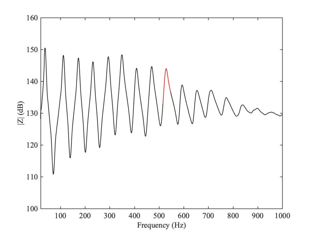
As we showed in section 10.5.1, each single term from the modal summation (1), when plotted in the Nyquist plane (real part of $Z$ versus imaginary part of $Z$), should give a circle. Figure 1 shows a typical measured input impedance function — this particular example is for a trombone, which we will study in section 11.5. A small section near one of the peaks has been highlighted in red. A Nyquist plot of that section gives the red curve in Fig. 2, and it does indeed look plausibly like an arc of a circle.
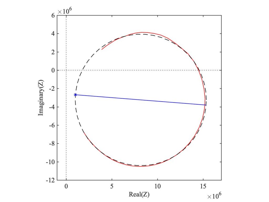
The fitting procedure now proceeds in two stages, both making use of the Matlab function “fminsearch”. The first stage is purely geometrical: the circle most closely approximating the red curve is found. The outputs of this stage are the $(x,y)$ coordinates of the centre, and the circle radius. The result, for our example, is the black dashed circle shown in Fig. 2. A graphical comparison like this allows the user to be sure that there really is only a single major peak in the selected frequency range — otherwise the circle would be distorted.
The second stage is to best-fit the parameters of a single term of equation (1) to the measured complex data, with the constraint that the result must lie on the circle found in the first stage. However, we need to make some allowance for the effect of all the other modes. Provided their resonance frequencies are well outside the frequency range we have chosen, the net effect of those contributions should be approximately a (complex) constant. The outputs of this stage are this complex constant, plus $\omega_m$, $Q_m$ and $A_m$ — but $A_m$ is allowed to be complex. The blue line in Fig. 2 indicates the fitted phase angle of $A_m$, and the blue star shows the point on the circle that would lie at the origin without the effect of the other modes.
Once this process has been carried out for all sufficiently strong peaks, equation (1) can be used to reconstruct $Z$ from the modal parameters. But at this stage we ignore the phases of the coefficients: if the pressure mode shapes of the tube are real, as we would expect provided the damping is fairly light, then the coefficients $A_m$ should all be positive real numbers, because each is the square of a modal amplitude at the measurement position. By this means, any errors in the measured phase of $Z$ are minimised.
What we actually need for our simulation algorithm is the impulse response corresponding to $Z$. Once we have our modal decomposition, there is a simple and explicit formula for that impulse response. Each term in equation (1) describes the frequency response function of a single degree of freedom oscillator (like a mass on a spring). We derived the impulse response for such an oscillator back in section 2.2.8. So we know that our impulse response $g(t)$ is given by
$$g(t) \approx \sum_m{A_m \cos(\omega_m t) e^{-\omega_m t/2Q_m}} \tag{2}$$
where, again, we use values of $A_m$ which are real and positive, ignoring the fitted phase.
Now we can describe the steps of a mode-based simulation. After a given number of time steps, we have available the stored history of the volume flow rate $v(t)$ into the reed mouthpiece. The resulting pressure inside the mouthpiece is then given by a convolution integral of the flow rate with the impulse response we have just found:
$$p(t) = \int_0^t{v(t-\tau) g(\tau) d \tau} . \tag{3}$$
The lower limit of the integral is written as $\tau=0$ here, on the assumption that the simulation started at time $t=0$. In any computer simulation we are really working in discrete time, so this integral is approximated by a sum. More important, we don’t actually need to do the potentially time-consuming convolution. Instead, as we saw back in section 9.5.2, we can use a recursive IIR filter to represent each term in the summation. This speeds things up, and means that we don’t in fact need to store the history of $v(t)$.
In this way, at a given time step in the simulation we calculate a new value for the pressure. If we are using the quasi-static reed model, all we have to do now is read off the corresponding new value of the volume flow rate from the reed characteristic, equation (9) from section 11.3.1. We use this new value to update all the IIR filters, and move on to the next time step. If we are taking account of the reed’s resonance, we have another IIR filter representing the reed motion, so we update that at each time step and then deduce the new value of volume flow rate as described at the end of section 11.3.1.