
We saw a preliminary account of the excitation mechanism in a clarinet, back in sections 8.5 and 8.5.3. That description was qualitatively correct, but no attempt was made at that stage to find a physically-correct form for the nonlinear valve characteristic of the mouthpiece and reed. Now we need to remedy that omission, to obtain a simulation model with plausible functional form and parameters that have a direct physical interpretation.
The situation is sketched in Fig. 1. The player provides a steady mouth pressure $p_m$, while the pressure $p(t)$ just inside the mouthpiece is varying in time: its evolution is the thing we are trying to simulate. Normally, $p_m > p$ so that there is a pressure difference across the narrow opening between reed and lay, through which air flows with a volume rate $v(t)$. For the simplest model, we can picture this narrow opening as being a rectangular slot of width $w$ and height $H$, so that the cross-sectional area is $wH$.

As the reed vibrates, $H$ will vary. It is convenient to write it as $H=H_0-y(t)$ where $H_0$ is the initial gap set by the player, and $y(t)$ is the inward displacement of the vibrating reed. But, as with other parameters in this model, $H$ and $y$ should be regarded as effective values, not necessarily exactly equal to distances you could directly measure. Some air will flow through the tapering gaps on the sides of the reed, for example, and this must be factored in to the effective area. Also, there is a fluid dynamical phenomenon called the vena contracta that can make the effective thickness of the air jet a bit less than the height of the opening.
Under the normal conditions of clarinet playing, it is a reasonable approximation to assume that the simplest form of Bernoulli’s law (see section 11.2.1) applies to the air jet. This assumption gives us a simple formula for the flow speed, and hence for the volume flow rate into the mouthpiece:
$$v=-w(H_0-y) \sqrt{2 |\Delta p|/\rho_0} \mathrm{~sign} (\Delta p) \tag{1}$$
where the pressure difference
$$\Delta p = p-p_m \tag{2}$$
and the term $\mathrm{sign}(\Delta p)$ serves to guarantee that the flow correctly reverses if the pressure difference should reverse. It might seem a little perverse to define the pressure difference this way, so that it is usually negative. But this form matches the way earlier plots were presented, for example in section 8.5, and it will be convenient for the later development of the simulation model. Note that in this derivation we have implicitly assumed that the flow speed $v$ is very small compared to the speed of sound. This is usually the case in normal woodwind playing, but in some extreme cases the local flow speed can get very high, and the approximation becomes questionable.
Now we need to think about the motion of the reed. The reed is essentially a cantilever beam, set into vibration by the time-varying pressure difference between the two faces. The reed will have many vibration resonances, of course, but it is sufficient for our purpose to include just the first of these. In that case, the reed displacement $y$ will behave like a damped harmonic oscillator, with a governing equation of the form
$$M_r \ddot{y} + C_r \dot{y} + K_r y=-\Delta p \tag{3}$$
where $M_r$ is the (effective) mass per unit area of the reed, $K_r$ is the corresponding effective stiffness per unit area, and $C_r$ is a damping coefficient per unit area. The resonance frequency $\omega_r$ will satisfy
$$\omega_r^2=K_r/M_r \tag{4}$$
as usual.
This resonance frequency for a typical clarinet reed and embouchure has been measured, and it is in the vicinity of 3 kHz. This means that playing frequencies of clarinet notes are almost invariably far lower than the reed resonance. In that case, the stiffness term of equation (3) will dominate, and we obtain the approximate result
$$K_r y \approx -\Delta p . \tag{5}$$
Eliminating $y$ in equation (1) then gives
$$v \approx -w\left(H_0+ \dfrac{\Delta p}{K_r}\right) \sqrt{2 \dfrac{|\Delta p|}{\rho_0}} \mathrm{~sign} (\Delta p) . \tag{6}$$
It is useful to introduce the closure pressure
$$p_c=K_r H_0 , \tag{7}$$
which is the minimum mouth pressure needed to close the reed completely against the lay, when the internal pressure $p=0$. We can then rewrite equation (6) in the form
$$v \approx -u_A\left(1+ \dfrac{\Delta p}{p_c}\right) \sqrt{\dfrac{|\Delta p|}{p_c}} \mathrm{~sign} (\Delta p) \tag{8}$$
where the constant
$$u_A = w H_0\sqrt{\dfrac{2 p_c}{\rho_0}} =w H_0^{3/2}\sqrt{\dfrac{2 K_r}{\rho_0}} . \tag{9}$$
Equation (8) is the nonlinear valve characteristic we are looking for. It is valid while $\Delta p > -p_c$, but at that point the reed closes. Once $\Delta p$ is more negative than this threshold, we have $v=0$.
The resulting nonlinear characteristic is plotted in the red curve of Fig. 2. The parameter values here are typical of a clarinet, according to the measurements of Dalmont and Frappé [1]: width $w$=15 mm, initial reed gap $H_0$=0.6 mm and closure pressure $p_c$=7 kPa. The corresponding reed stiffness is $K_r$=12.7 kPa/mm. Dalmont and Frappé also show direct measurements of the steady flow characteristics of a clarinet reed and mouthpiece, demonstrating excellent agreement with the functional form of equation (8) (despite the approximations we have used in order to derive this equation).
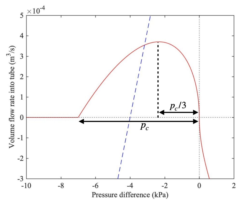
The dashed blue line in Fig. 2 shows a typical example of the sloping straight line whose intersection with the red curve forms a key part of the simulation model (see section 8.5.3 for the details). The slope of this line is $1/Z_t$ where $Z_t=\rho_0 c/S$ is the characteristic impedance of the tube. The cross-sectional area $S$ used here is based on the typical bore diameter of a clarinet tube, 15 mm. Notice that this sloping line is significantly steeper than the maximum slope of the red curve. We can deduce that for this model clarinet there will be no equivalent of the “Friedlander ambiguity” that we found for a bowed string, in which the corresponding sloping line could sometimes intersect the nonlinear friction curve at three points rather than one, leading to the “flattening effect” (see section 9.2).
For $\Delta p > -p_c$ we can rewrite equation (8) as
$$v \approx u_A\left(1+ \dfrac{p-p_m}{p_c}\right) \sqrt{\dfrac{p_m-p}{p_c}} .\tag{10}$$
Differentiating this equation gives
$$\dfrac{dv}{dp}= -\dfrac{u_A}{2p_c} \left(\dfrac{p_m-p}{p_c}\right)^{-1/2} +\dfrac{3u_A}{2p_c} \left(\dfrac{p_m-p}{p_c}\right)^{1/2}$$
$$=\dfrac{u_A}{2p_c} \left(\dfrac{p_m-p}{p_c}\right)^{-1/2} \left[-1 + 3\left( \dfrac{p_m-p}{p_c} \right) \right] . \tag{11}$$
The maximum of the curve, where this slope is zero, is thus defined by
$$\dfrac{p_m-p}{p_c}=\dfrac{1}{3} \tag{12}$$
as indicated by the dotted line in Fig. 2. At this value of $\Delta p$, the value of the volume flow rate is
$$v_{max}=\dfrac{2u_A}{3 \sqrt{3}} . \tag{13}$$
If we want a time-stepping simulation model which includes the reed resonance, we need to go back to equations (1) and (3) to see how to proceed. At each time step of the simulation, we first compute a new value for the reed displacement $y$. The most efficient way to do this, based on the history of the forcing term $-\Delta p$, is to use a recursive IIR digital filter, as described in section 9.5.2. If this calculation gives a value $y > H_0$, then in fact the reed closes at that moment and we use $y=H_0$ instead.
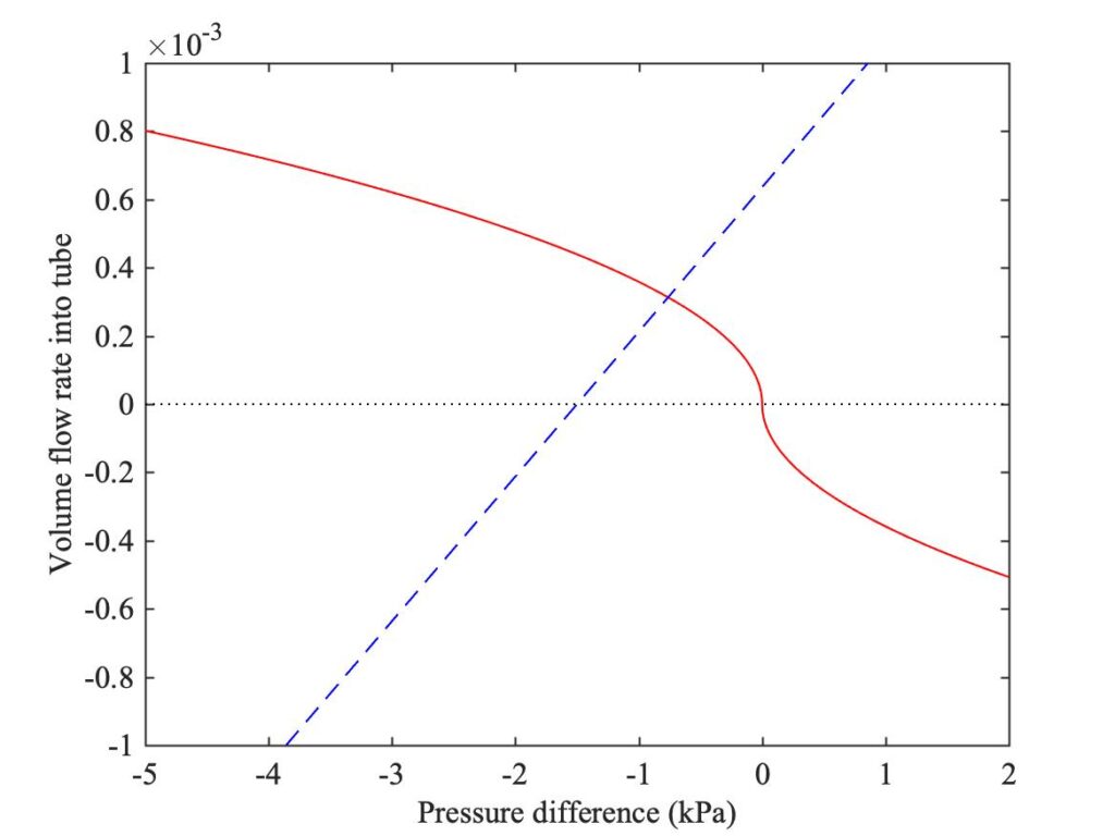
Now we use equation (1) with this value of $y$, which gives a different nonlinear function of pressure $p$: the factor $(H_0-y)$ is now a known constant, and only the square root term gives non-trivial variation with $p$. We thus need to find the intersection of this new function with the sloping straight line, to give the new values of $p$ and $v$: an example is shown in Fig. 3. The rest of the simulation model is unchanged: we still use convolution with a reflection function to model the linear acoustics of the tube, and give a value of $p_h$ which determines the position of the sloping straight line.
There is one final thing to mention. The flow of air through the reed gap given by equation (1) is not the only contribution to the total volume flow rate into the instrument. The reed also induces a “sweeping flow” component by its own motion. For a reed of the kind we are looking at here, that contribution to the inward volume flow rate is proportional to the reed tip velocity $\dot{y}$, scaled by an “effective reed area” $A_r$, so that equation (1) becomes
$$v=-w(H_0-y) \sqrt{2 |\Delta p|/\rho_0} \mathrm{~sign} (\Delta p)+A_r \dot{y} . \tag{14}$$
We will neglect this extra term for now, in the interests of simplicity, but we will need to include it in later sections when we discuss some subtleties of brass and free reed instruments.
[1] Jean-Pierre Dalmont and Cyrille Frappé, “Oscillation and extinction thresholds of the clarinet: Comparison of analytical results and experiments”, Journal of the Acoustical Society of America 122, 1173—1179 (2007).